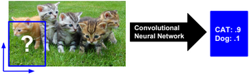
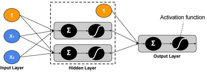
A neural network is a non-linear classifier (separator is not a linear function). It can also be used for regression.
A Shallow neural network is a one hidden layer neural network.
A Vanilla neural network is a regular neural network having layers that do not form cycles.
TensorFlow Playground is an interactive web interface for learning neural networks: http://playground.tensorflow.org.
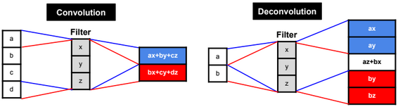
Computational Graph
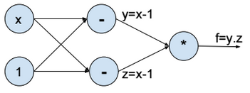
Above the computational graph for the function \(f(x) = (x-1)^2\).
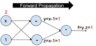
Forward propagation
To minimize the function f, we assign a random value to x (e.g. x = 2), then we evaluate y, z, and f (forward propagation).
Backward propagation
Then we compute the partial derivative of f with respect to x step by step (Backward propagation).
\(\frac{\partial f}{\partial x} = \frac{\partial f}{\partial y}*\frac{\partial y}{\partial x} + \frac{\partial f}{\partial z}*\frac{\partial z}{\partial x} = 2 \\ \frac{\partial f}{\partial y} = z = 1 \\ \frac{\partial f}{\partial z} = y = 1 \\ \frac{\partial y}{\partial x} = \frac{\partial z}{\partial x} = 1\)
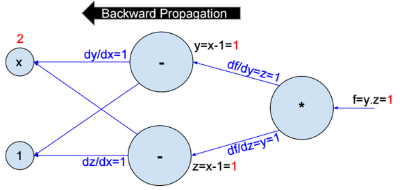
Then we update \(x:= x – ?.\frac{\partial f}{\partial x}\).
We repeat the operation until convergence.
Activation functions
Activation functions introduce nonlinearity into models. The most used activation functions are:
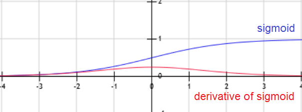
Sigmoid
\(f(x) = \frac{1}{1+exp(-x)}\)
Sigmoid has a positive and non-zero centred output (sigmoid(0) ? 0.5).
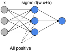
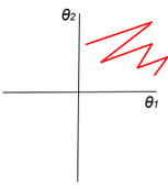
When all activation units are positive, then weight update will be in the same direction (all positive or all negative updates) and that will cause a zigzag path during optimization.
\(z=?w_i.a_i+b \\ \frac{dL}{dw_i}=\frac{dL}{dz}.\frac{dz}{dw_i}=\frac{dL}{dz}.ai\)
If all ai>0, then the gradient will have the same sign as \(\frac{dL}{dz}\) (all positive or all negative).
TanH
\(f(x) = \frac{2}{1+exp(-2x)} -1\)
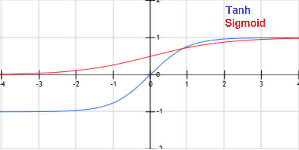
When x is large, the derivative of the sigmoid or Tanh function is around zero (vanishing gradient/saturation).
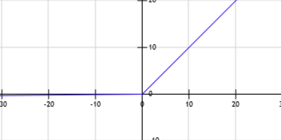
ReLU (Rectified Linear Unit)
f(x) = max(0, x)
Leaky ReLU
f(x) = max(0.01x, x)
Leaky Relu was introduced to fix the ôDying Reluö problem.
\(z=?w_i.a_i+b \\ f=Relu(z) \\ \frac{dL}{dw_i}=\frac{dL}{df}.\frac{df}{dz}.\frac{dz}{dw_i}\)
When z becomes negative, then the derivative of f becomes equal to zero, and the weights stop being updated.
PRelu (Parametric Rectifier)
f(x) = max(?.x, x)
ELU (Exponential Linear Unit)
f(x) = {x if x>0 otherwise ?.(exp(x)-1)}
Other activation functions: Maxout
Cost function
\(J(?) = \frac{1}{m} \sum_{i=1}^{m} loss(y^{(i)}, f(x^{(i)}; ?))\)
We need to find ? that minimizes the cost function: \(\underset{?}{argmin}\ J(?)\)
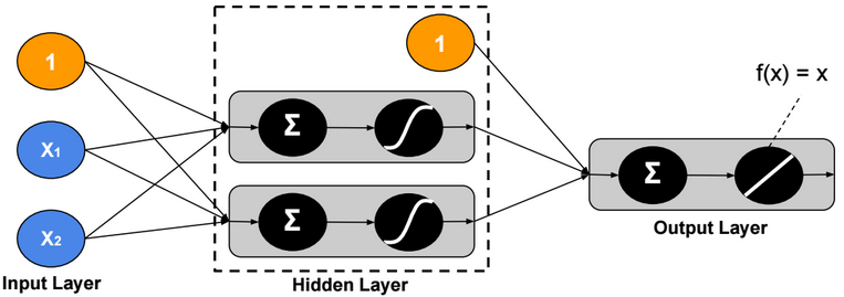
Neural Network Regression
Neural Network regression has no activation function at the output layer.
L1 Loss function
\(loss(y,?) = |y – ?|\)
L2 Loss function
\(loss(y,?) = (y – ?)^2\)
Hinge loss function
Hinge loss function is recommended when there are some outliers in the data.
\(loss(y,?) = max(0, |y-?| – m)\)
Two-Class Neural Network
Binary Cross Entropy Loss function
\(loss(y,?) = – y.log(?) – (1-y).log(1 – ?)\)
Multi-Class Neural Network – One-Task
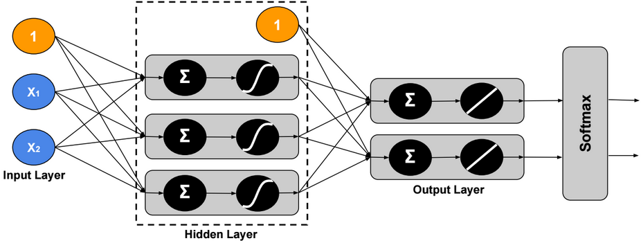
Using Softmax, the output ? is modeled as a probability distribution, therefore we can assign only one label to each example.
Cross Entropy Loss function
\(loss(Y,\widehat{Y}) = -\sum_{j=1}^c Y_{j}.log(\widehat{Y}_{j})\)
Hinge Loss (SVM) function
\(y = \begin{bmatrix} 1 \\ 0 \\ 0 \end{bmatrix},\ ? = \begin{bmatrix} 2 \\ -5 \\ 3 \end{bmatrix} \\ loss(y,?) = \sum_{c?1} max(0, ?_c – ?_1 + m)\)
For m = 1, the sum will be equal to 2.
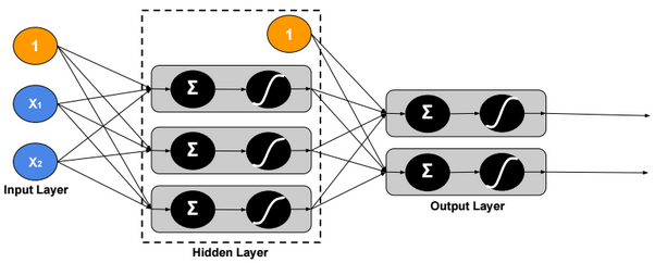
Multi-Class Neural Network – Multi-Task
In this version, we assign multiple labels to each example.
Loss function
\(loss(Y,\widehat{Y}) = \sum_{j=1}^c – Y_j.log(\widehat{Y}_j) – (1-Y_j).log(1 – \widehat{Y}_j)\)
Regularization
Regularization is a very important technique to prevent overfitting.
Dropout
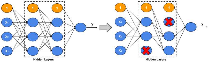
For each training example, ignore randomly p activation nodes of each hidden layer. p is called dropout rate (p?[0,1]). When testing, scale activations by the dropout rate p.
Inverted Dropout
With inverted dropout, scaling is applied at the training time, but inversely. First, dropout all activations by dropout factor p, and second, scale them by inverse dropout factor 1/p. Nothing needs to be applied at test time.
Data Augmentation
As a regularization technique, we can apply random transformations on input images when training a model.
Early stopping
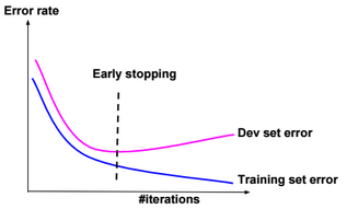
Stop when error rates decreases on training data while it increases on dev (cross-validation) data.
L1 regularization
\(J(?) = \frac{1}{m} \sum_{i=1}^{m} loss(y^{(i)}, f(x^{(i)}; ?)) \color{blue} { + ? .\sum_{j} |?_j|} \)
? is called regularization parameter
L2 regularization
\(J(?) = \frac{1}{m} \sum_{i=1}^{m} loss(y^{(i)}, f(x^{(i)}; ?)) \color{blue} { + ? .\sum_{j} ?_j^2} \)
Lp regularization
\(J(?) = \frac{1}{m} \sum_{i=1}^{m} loss(y^{(i)}, f(x^{(i)}; ?)) \color{blue} { + ? .\sum_{j} ?_j^p} \)
For example, if the cost function \(J(?)=(?_1 – 1)^2 + (?_2 – 1)^2\), then the \(L_2\) regularized cost function is \(J(?)=(?_1 – 1)^2 + (?_2 – 1)^2 + ? (?_1^2 + ?_2^2)\)
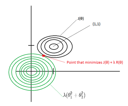
If ? is large, then the point that minimizes the regularized J(?) will be around (0,0) –> Underfitting.
If ? ~ 0, then the point that minimizes the regularized J(?) will be around (1,1) –> Overfitting.
Elastic net
Combination of L1 and L2 regularizations.
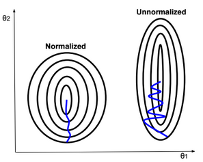
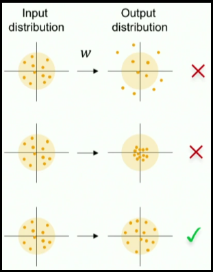
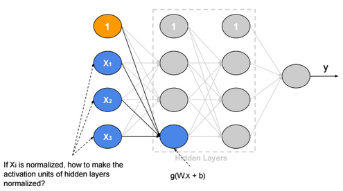
Normalization
Gradient descent converges quickly when data is normalized Xi ? [-1,1]. If features have different scales, then the update of parameters will not be in the same scale (zig-zag).
For example, if the activation function g is the sigmoid function, then when W.x+b is large g(W.x+b) is around 1, but the derivative of the sigmoid function is around zero. For this reason the gradient converges slowly when the W.x+b is large.
Below some normalization functions.
ZScore
\(X:= \frac{X – ?}{?}\)
MinMax
\(X:= \frac{X – min}{max-min}\)
Logistic
\(X:= \frac{1}{1+exp(-X)}\)
LogNormal
\(X:= \frac{1}{?\sqrt{2?}} \int_{0}^{X} \frac{exp(\frac{-(ln(t) – ?)^2}{2?^2})}{t} dt\)
Tanh
\(X:= tanh(X)\)
Weight Initialization
Weight initialization is important because if weights are too big then activations explode. If weights are too small then gradients will be around zero (no learning).
When we normalize input data, we make the mean of the input features equals to zero, and the variance equals to one. To keep the activation units normalized too, we can initialize the weights \( W^{(1)}\) so \(Var(g(W_{j}^{(1)}.x+b_{j}^{(1)}))\) is equals to one.
If we suppose that g is Relu and \(W_{i,j}, b_j, x_i\) are independent, then:
\(Var(g(W_{j}^{(1)}.x+b_{j}^{(1)})) = Var(\sum_{i} W_{i,j}^{(1)}.x_i+b_{j}^{(1)}) =\sum_{i} Var(W_{i,j}^{(1)}.x_i) + 0 \\ = \sum_{i} E(x_i)^2.Var(W_{i,j}^{(1)}) + E(W_{i,j}^{(1)})^2.Var(x_i) + Var(W_{i,j}^{(1)}).Var(x_i) \\ = \sum_{i} E(x_i)^2.Var(W_{i,j}^{(1)}) + E(W_{i,j}^{(1)})^2.Var(x_i) + Var(W_{i,j}^{(1)}).Var(x_i) \\ = \sum_{i} 0 + 0 + Var(W_{i,j}^{(1)}).Var(x_i) = n.Var(W_{i,j}^{(1)}).Var(x_i) \)
Xavier initialization
If we define \(W_{i,j}^{(1)} ? N(0,\frac{1}{\sqrt{n}})\), then the initial variance of activation units will be one (n is number of input units).
We can apply this rule on all weights of the neural network.
Batch Normalization
Batch normalization is a technique to provide any layer in a Neural Network with normalized inputs. Batch Normalization has a regularizing effect.
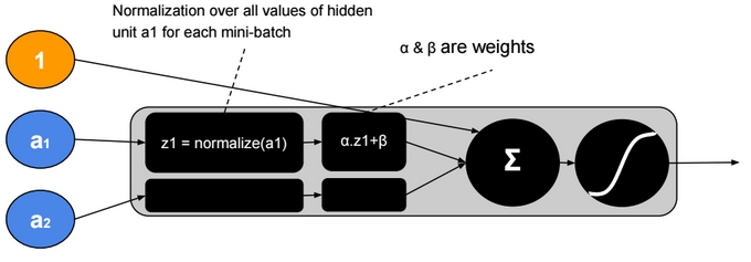
After training, ? will converge to the standard deviation of the mini-batches and ? will converge to the mean. The ?, ? parameters give more flexibility when shifting or scaling is needed.
Hyperparameters
Neural network hyperparameters are:
- Learning rate (?) (e.g. 0.1, 0.01, 0.001,…)
- Number of hidden units
- Number of layers
- Mini-bach size
- Momentum rate (e.g. 0.9)
- Adam optimization parameters (e.g. ?1=0.9, ?2=0.999, ?=0.00000001)
- Learning rate decay
Local Minimum
The probability that gradient descent gets stuck in a local minimum in a high dimensional space is extremely low. We could have a saddle point, but itĺs rare to have a local minimum.
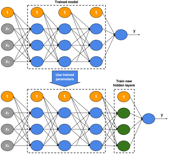
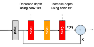
Transfer Learning
Transfer Learning consists in the use of parameters of a trained model when training new hidden layers of an extended version of that model.