Quantile Regression

Similar to Linear Regression, Quantile Regression estimates the conditional median instead of the conditional mean.

Decision Tree

Decision Tree is a classification algorithm.

Information Gain

Given the following training set {S}:

X1	X2	Y
a	c	e
a	d	e
b	d	f
b	d	f

We need to define the first level of the decision tree by choosing one of the two features x1 or x2. We need to calculate the Information Gain (I) for each case, and select the feature with higher Information Gain.

\(I(x) = Entropy(parent) – Expected Entropy(children) \) \(I(X1) = 1 – 0\) \(I(X2) = 1 – 0.688\)

When training the model, always use data with equal number of rows for each output, so the entropy of the root node equals to 1. (Entropy measure the uncertainty of the data).

Each node of the tree defines a probability estimation for each output.

More details: https://www.youtube.com/watch?v=-dCtJjlEEgM

Standard Deviation Reduction

Another approach to select features that define the levels of a decision tree is by calculating the Standard Deviation Reduction.

Boosted Decision Tree

A boosted decision tree is an ensemble learning method in which the second tree corrects for the errors of the first tree, the third tree corrects for the errors of the first and second trees, and so forth. The data points which were misclassified receives a bigger weight in the data, the ones correctly classified received a diminished weight. The idea is that with each iteration, the data points misclassified have increasing importance, allowing the learner to fit better and improve accuracy.

Predictions are based on the entire ensemble of trees together that makes the prediction.

Random Forest

When we have thousand of features (d), calculating the Information Gains for each split point and for each feature requires a lot of time and resources.

The idea in the Random Forest algorithm is to:

1-select a subset of size N from the training data

2-Pick up randomly k features, project the data on the k features, and select the split point with higher information gain.

Repeat step 2 until the creation of the tree (we can stop the operation at a certain depth of tree).

Repeat step 1 and 2 to generate more trees.

For a new example, we push it through all trees until it reaches the corresponding leaves. then we calculate the probability as the average of probabilities generated by all trees:

\(P(y=k|x) = \frac{1}{nbr\ trees} \sum_{t=1}^{nbr\ trees} P_t(y=k|x)\)

Clean Missing Data

How estimate missing data?

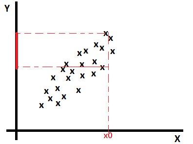
We can replace missing data with the Mean, the Median or the Mode, but usually it’s not an efficient approach.

If data are multi-variable distributed as below, if there is an example (x0, ?) with a missing value y, we can estimate y as a mean of values y for examples having x near to x0.

Linear regression based imputation

Find a model that estimates missing values based on other features: \(missing\_value = ?_0 + ?_1 * x_1 + ?_2 * x_2 + … + ?_{n+1} * y\)

MICE (Multiple Imputation through Chained Equations)

1-Replace all missing values with random values.

2-Pick randomly a value from one of the three nearest examples. The distance is calculated on values predicted using a regression function(linear, logistic, multinomial). Run the operation for each missing value.

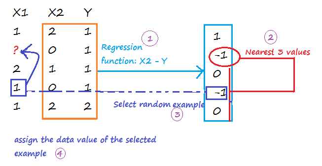
Repeat step 1 and 2 m times to create m imputed data sets. Calculate the mean of imputed values from all imputed data sets, and assign it to each missing value of the original data set.

Probabilistic PCA

The PCA approach is based on the calcul of a low-dimensional approximation of the data, from which the full data is reconstructed. The new reconstructed matrix is used to fill missing values.

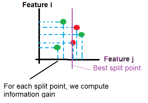
Filter based Feature Selection

Pearson Correlation

Pearson correlation coefficient:

\( r_{X,Y} = \frac{Cov(X,Y)}{?_X * ?_Y} \in [-1, 1]\)

Strong positive correlation when \(r_{X,Y}\) around 1.

No correlation when \(r_{X,Y}\) around 0.

Strong negative correlation when \(r_{X,Y}\) around -1.

Mutual Information

\(I(X,Y) = \sum_{x,y} p(x,y)*log(\frac{p(x,y)}{p(x)*p(y)}) >= 0\)

I(X,Y) = 0 when X, Y are independent

Kendall Correlation

Kendall correlation coefficient:

\(? = \frac{C-D}{C+D} \in [-1, 1]\)

C is the number of concordant pairs

D is the number of discordant pairs

X1 (Sorted)	X2	C	D
1	2	#values{X2>2 && X1>1}=3	#values{X2<2 && X1>1}=1
2	1	#values{X2>1 && X1>2}=3	#values{X2<1 && X1<2}=0
3	3	#values{X2>3 && X1>3}=2	#values{X2<3 && X1<3}=0
4	5	#values{X2>5 && X1>4}=0	#values{X2<5 && X1<4}=1
5	4	#values{X2>4 && X1>5}=0	#values{X2<4 && X1<5}=0
Total		8	2

\(? = \frac{C-D}{C+D} = 0.6\) (Good correlation)

For more details: https://www.youtube.com/watch?v=oXVxaSoY94k

Spearman Correlation

Spearman Correlation coefficient:

The Spearman correlation coefficient is defined as the Pearson correlation coefficient between the ranked variables.

\(r_S = \frac{Cov(rg\_X,rg\_Y)}{?_{rg\_X} * ?_{rg\_X}} \in [-1, 1]\)

X	Y	rg_X (X rank)	rg_Y (Y rank)
1	2	1	2
3	1	2	1
4	4	3	3
6	7	4	4
10	9	5	5

\(r_S = \frac{Cov(rg\_X,rg\_Y)}{?_{rg\_X} * ?_{rg\_Y}} = 0.8\)

Chi-Squared

Example:

X1	X2
1	2
3	1
3	1
3	1
3	2
3	2

Occurence X1/X2	1	2
1	0 (3/6)	1 (3/6)
2	0 (0/6)	0 (0/6)
3	3 (15/6)	2 (15/6)

In bold the expected value ((row total*column total)/n).

\(\chi^2 = \frac{(1-3/6)^2}{3/6} + \frac{(0-3/6)^2}{3/6} + \frac{(3-15/6)^2}{15/6} + \frac{(2-15/6)^2}{15/6}=1.2\)

Fisher Score

I don’t know the exact formula used, maybe the coefficient is calculated as below:

\( r = \frac{\sum_{i=1}^{n} (X_i – \overline{X})*(Y_i – \overline{Y})}{\sqrt{(\sum_{i=1}^{n} (X_i – \overline{X})^2) * (\sum_{i=1}^{n} (Y_i – \overline{Y})^2)}}\)

http://www.wikiwand.com/en/Fisher_transformation

Count-Based

Count of values for each feature.

Skewed Data

When training data are imbalanced (skewed), machine learning algorithms tend to minimize errors for the majority classes on the detriment of minority classes. It usually produces a biased classifier that has a higher predictive accuracy over the majority classes, but poorer predictive accuracy over the minority classes.

Synthetic Minority Oversampling Technique (SMOTE)

SMOTE is an algorithm that creates extra training data by performing certain operations on real data.

Given a set S = {(0,A), (1,A), (2,A), (3,A), (4,B), (5,B)}, A is the majority class, and B the minority class. If the amount of over-sampling needed is 200% (2x) and the number of nearest neighbors is 2, then the algorithm generates new samples in the following way:

Take the difference between an example under consideration and one of its nearest neighbor. Multiply this difference by a random number between 0 and 1, and add it to the feature vector under consideration.

Existing example (4,B) –> New example (4 + 0.3*(4-5), B)

Model Evaluation

Metrics

Mean Absolute Error	\(\frac{1}{m} \sum_{i=1}^{m} |y – h_?(x)|\)
Root Mean Squared Error (the standard deviation of the distribution of errors)	\(\sqrt{\frac{1}{m} \sum_{i=1}^{m} (y – h_?(x))^2} = \sqrt{J(?)}\)
Relative Absolute Error	\(\frac{\sum_{i=1}^{m} |y – h_?(x)|}{\sum_{i=1}^{m} |y – \frac{\sum_{i=1}^{m} y}{m}|}\)
Relative Squared Error	\(\frac{\sum_{i=1}^{m} (y – h_?(x))^2}{\sum_{i=1}^{m} (y – \frac{\sum_{i=1}^{m} y}{m})^2}\)
Coefficient of Determination (\(R^2\))	1 – [Relative Squared Error]

True Positive: \(1\{y=1, h_?(x)=1\}\)

False Positive: \(1\{y=0, h_?(x)=1\}\)

True Negative: \(1\{y=0, h_?(x)=0\}\)

False Negative:\(1\{y=1, h_?(x)=0\}\)

Accuracy	\(\frac{[True Positive] + [True Negative]}{m}\)
Precision	\(\frac{[True Positive]}{[True Positive] + [False Positive]}\)
Recall	\(\frac{[True Positive]}{[True Positive] + [True Negative]}\)
F1 Score	\(2 \frac{[Precision]*[Recall]}{[Precision]+[Recall]}\)

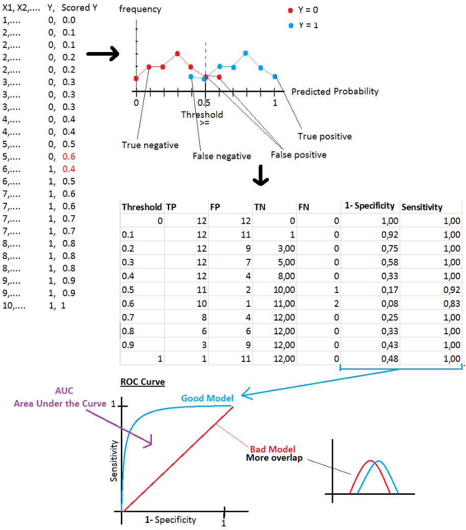
ROC Curve

Specificity: True Negative / (True Negative + False Positive)

Sensitivity: True Positive / (True Positive + False Negative)

AzureML components

Data Format Conversions

Convert to Dataset

Data Input/Output

Enter Data Manually
Import Data	Import from: Azure Block Storage, Azure SQL Database, Azure Table, Hive Query, Web URL, Data Feed Provider(OData), Azure DocumentDB
Export Data

Data Transformation

Edit Metadata	Rename columns
Join Data
Select Columns in Dataset
Remove Duplicate Rows
Slit Data
Partition and Sample	Select Top xxx rows, or generate a sample, or split data in k folds
Group Data into Bins
Clip Value	Remove outliers (peak and subpeak)
Build Counting Transform	For each selected column, and for an output class, calculate the occurrence of a value in all rows. Example: Country Product Advertised (2 classes) Country Class 0 Count Country Class 1 Count Product Class 0 Count Product Class 1 Count FR P1 0 1 0 2 1 CA P1 0 1 2 2 1 CA P1 1 1 2 2 1 CA P2 1 1 2 0 1 Note: On AzureML, we get wrong results if the number of rows is low.

Statistical Functions

Summarize Data

Machine Learning

Train Model
Tune Model Hyperparameters	Find best hyperparameter values
Score Model
Evaluate Model	Evaluate and compare one or two scored datasets
Train Clustering Model

R/Python Language Modules

Create R Model
Execute R Script
Execute Python Script	Supported Python packages: NumPy, pandas, SciPy, scikit-learn, matplotlib

Machine Learning Methods

Anomaly Detection Algorithms

One-Class SVM	The algorithm finds a minimal hypersphere around the data. Any point outside the hypersphere is considered an outlier.
PCA-Based Anomaly Detection	The algorithm applies PCA to reduce the dimensionality of the data, and applying distance metrics to identify cases that represent anomalies.

Classification Algorithms

Logistic Regression
Neural Network
Averaged Perceptron	Averaged Perceptron algorithm is an extension of the standard Perceptron algorithm; it uses averaged weights and biases.
Bayes Point Machine	It’s Bayesian linear classifier, therefore the model is not prone to overfitting
Decision Forest
Decision Jungle
Boosted Decision Tree
Decision Forest
Decision Jungle
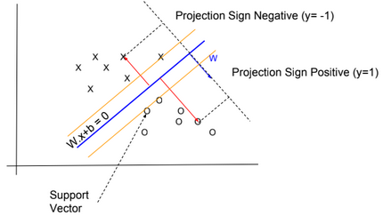
SVM	The algorithm finds an optimal hyperplane that categorizes new examples. I didn’t know which kernel function is used by the algorithm. Probably it uses a linear kernel \(K(x,x’) = x^T .x’)\) SVM is not recommended with large training sets, because the classification of new examples requires the computation of kernels using all training examples.
Locally Deep SVM	The algorithm defines a tree to cluster examples (like Decision Tree algorithm), and then trains SVM on each cluster.
One-vs-All Multiclass	The One-vs-All Multiclass requires as an input multiple two-class classification algorithms. To classify a new example, the algorithm runs two-class classification algorithms for each class, then select the class with higher probability.

Clustering Algorithms

K-Means Clustering

Regression Algorithms

Bayesian Linear Regression	This model is not prone to overfitting
Boosted Decision Tree Regression
Decision Forest Regression
Fast Forest Quantile Regression
Neural Network Regression	Neural network with an output layer having no logistic function
Linear Regression
Ordinal Regression	Algorithm used for predicting an ordinal variable.
Poisson Regression	Algorithm used for predicting a Poisson variable