Architecture
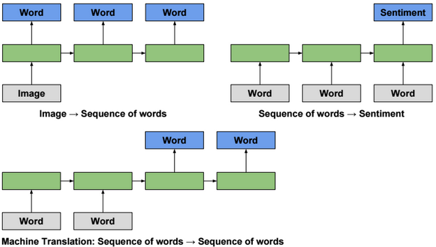
RNNs are generally used for sequence modeling (e.g. language modeling, time series modeling,…).
Unfolding a RNN network (many to many scenario) could be presented as follow:

When training the model, we need to find W that minimizes the sum of losses.
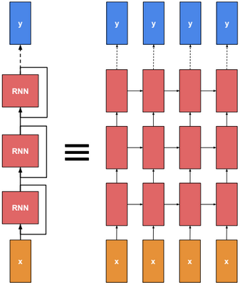
Multilayer RNN
Multilayer RNN is a neural network with multiple RNN layers.
Backpropagation through time
To train a RNN, we need to calculate the gradient to update parameters. Instead of doing the derivations for the full network, we will focus only on one hidden unit.
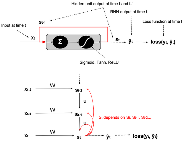
We define \(s_t = g(W.x_t + U.s_{t-1} + b) \). g is an activation function.
Using the chain rule we can find that:
\(\frac{\partial loss(y_t,?_t)}{\partial W} = \frac{\partial loss(y_t,?_t)}{\partial ?_t}.\frac{\partial ?_t}{\partial s_t}.\frac{\partial s_t}{\partial W} \\ = \frac{\partial loss(y_t,?_t)}{\partial ?_t}.\frac{\partial ?_t}{\partial s_t}.(\sum_{k=t}^0 \frac{\partial s_t}{\partial s_k}.\frac{\partial s_k}{\partial W})\)Vanishing gradient
The term in red in the equation is a product of Jacobians (\(\frac{\partial s_t}{\partial s_k} = \prod_{i=k+1}^{t} \frac{\partial s_{i}}{\partial s_{i-1}}\)).
\(\frac{\partial loss(y_t,?_t)}{\partial ?_t}.\frac{\partial ?_t}{\partial s_t}.(\sum_{k=t}^0 \color{red} {\frac{\partial s_t}{\partial s_k}}.\frac{\partial s_k}{\partial W})\)Because the derivatives of activation functions (except ReLU) are less than 1, therefore when evaluating the gradient, the red term tends to converge to 0, and the model becomes more biased and captures less dependencies.
Exploding gradient
RNN is trained by backpropagation through time. When gradient is passed back through many time steps, it tends to vanish or to explode.
Gradient Clipping
Gradient Clipping is a technique to prevent exploding gradients in very deep networks, typically Recurrent Neural Networks. There are various ways to perform gradient clipping, but the most common one is to normalize the gradients of a parameter vector when its L2 norm exceeds a certain threshold according to : \(gradients := gradients * \frac{threshold}{L2 norm(gradients)}\).
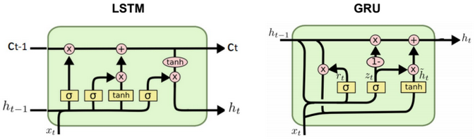
Long Short Term Memory (LSTM)
LSTM was introduced to solve the vanishing gradient problem.
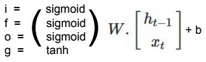
In LSTM, there are 4 gates that regulate the state of a RNN model:
Write gate (i?[0,1]) (Input gate): Write to memory cell.
Keep gate (f?[0,1]) (Forget gate): Erase memory cell.
Read gate (o?[0,1]) (Output gate): Read from memory cell.
Gate gate (g?[-1,1]) (Update gate) How much to write to memory cell.
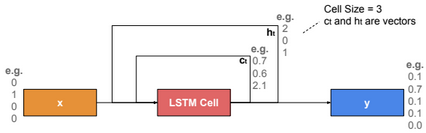
\(c_t\) is called memory state at time t.
i,f,o,g,h,c are vectors having the same size. W is a matrix with size nxh.
The gate states are calculated using the following formula:
The output \(h_t\) is calculated using the following formulas:
\(c_t = f.c_{t-1} + i.g \\ h_t = o.tanh(c_t)\)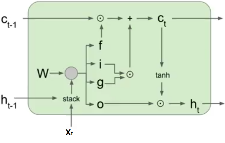
Gated Recurrent Unit (GRU)
The Gated Recurrent Unit is a simplified version of an LSTM unit with fewer parameters. Just like an LSTM cell, it uses a gating mechanism to allow RNNs to efficiently learn long-range dependency by preventing the vanishing gradient problem. The GRU consists of a reset and update gates that determine which part of the old memory to keep or update with new values at the current time step.