SSAS Architecture
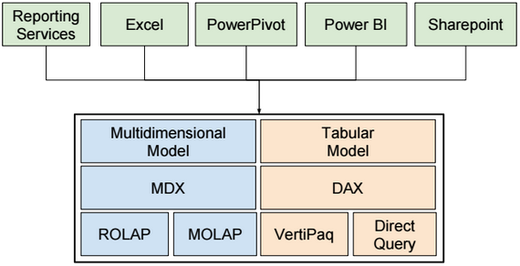
SSAS Server Modes
There are three SSAS Server Modes: Multidimensional, Tabular and Sharepoint.
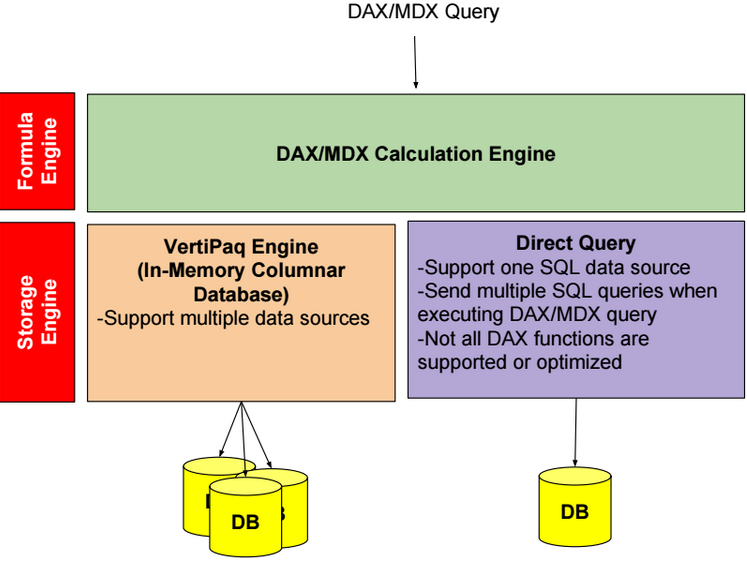
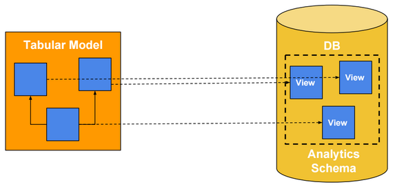
SSAS Tabular Architecture
Tabular Model
It’s recommended to use views instead of tables when adding tabular model tables.
View names, column names and tabular table/column names should be user friendly.
For example, use “Customer”, “Sales” and “Quantity” instead of “DimCustomer”, “FactSales” and “Sum of Quantity”.
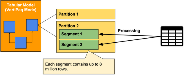
Vertipaq Mode
When processing in-memory partitions, data are loaded and processed by segment. Each segment contains up to 8 millions rows. Each segment is compressed and stored in memory. Uncompressed data are deleted.
Parallel processing of partitions requires more memory than sequential processing.
The number or rows per segment can be changed by specifying a value for the server property DefaultSegmentRowCount.
To monitor memory usage by model object, we can use the following Data Management Views (DMV) tables:
SELECT * FROM $System.discover_storage_table_columns
VertiPaq Compression
VertiPaq compression algorithms aim to reduce memory usage of tabular models. There are 3 main encoding algorithms:
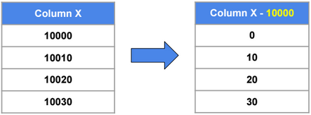
Value Encoding
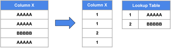
Dictionary Encoding
Run Length Encoding (RLE)
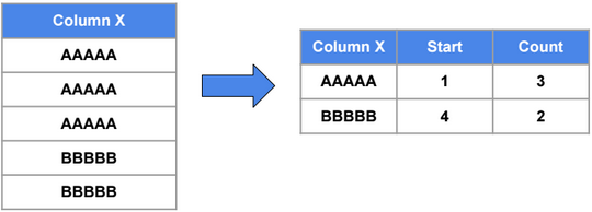
Partitioning
Partitioning does not improve performance, but it simplifies manageability.
It’s recommended to have one or many partitions with size equals to one or many segment sizes (e.g. 16M/24M/… rows).
Processing
Below SSAS processing options:
|
Process Clear |
Drops all the data in a database, table, or partition. |
|
Process Full |
Loads data into all selected partitions or tables. Any affected calculated columns, relationships, user hierarchies, or internal engine structures (except table dictionaries) are recalculated. |
|
Process Data |
Loads data into a partition or table without recalculating calculated columns. |
|
Process Recalc |
For all tables in the database, recalculates calculated columns, rebuilds relationships, rebuilds user hierarchies, and rebuilds other internal engine structures. Table dictionaries are not affected. |
|
Process Add |
Adds rows to a partition. Any affected calculated columns, relationships, user hierarchies, or internal engine structures (except table dictionaries) are recalculated. Each Process Add creates a new segment. |
|
Process Default |
Loads data into unprocessed partitions or tables. Any affected calculated columns, relationships, user hierarchies, or internal engine structures (except table dictionaries) are recalculated. |
|
Process Defrag |
Optimizes a table dictionary (an internal engine structure) for a given table or for all tables in the database. |
Use maxParallelism in the TMSL processing script to limit the number of parallel processing
{
“sequence”: {
“maxParallelism” : 2,
“operations” : [ { “refresh” : { “type” : “automatic”, “objects” : [ { “database” : “TabularProject” }]}}]
}.
Hardware Configuration
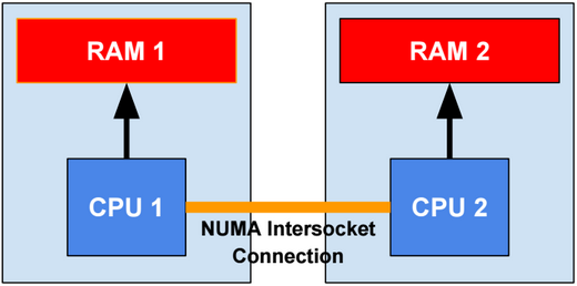
CPU and Memory performance are the most important factors when choosing a hardware.
SSAS 2016 SP1 is NUMA-aware. Being NUMA aware means that SSAS tries to reduce at a minimum the usage of the NUMA intersocket connection by preferring the usage of the local RAM bus.
Memory Management
Below server properties related to memory management:
|
VertiPaqPagingPolicy |
Enable/disable memory paging. |
|
VertiPaqMemoryLimit (in percentage or in number of bytes) |
VertiPaq memory limit to store the data (cache excluded). |
|
TotalMemoryLimit (in percentage or in number of bytes) |
Maximum memory that can be used by the SSAS server. |
|
LowMemoryLimit (in percentage or in number of bytes) |
A lower threshold at which the server first begins releasing memory allocated to infrequently used objects. |
|
HardMemoryLimit (in percentage or in number of bytes) |
A threshold at which Analysis Services begins rejecting requests outright due to memory pressure. |
We can use Performance Monitor tool to track memory usage.
Performance Monitoring
The two main tools we can use to monitor performance are Sql Profiler and Extended Events.
When using Extended Events, we need to set AutoRestart to true, so after a restart of the SSAS server, the capture of extended events automatically starts.
Direct Query Mode
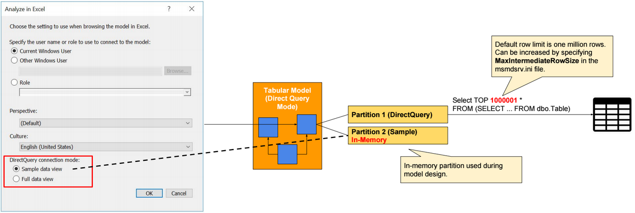
In Direct Query mode, we can create Direct Query partitions and Sample partitions. Direct Query partitions are not stored in-memory. Sample partitions are In-memory partitions, and they are used only during model design. Sample partitions require processing.
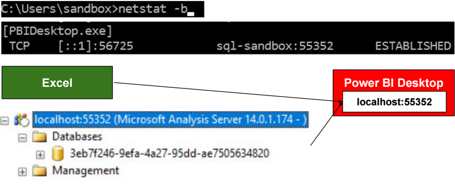
From Excel, we can select between using data from Sample partitions or from Direct Query partitions. This option is available when we open Excel from a Tabular model opened in Visual Studio.
In Direct Query mode, if row-level security is defined in data source tables, then we need to configure SSAS to delegate the identity of users when querying data source tables. SSAS can impersonate a Windows user, only when Kerberos Constrained Delegation (KCD) is configured.
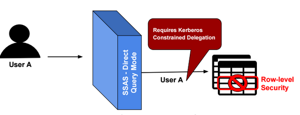
More details about Kerberos Constrained Delegation configuration can be found in the following link:
https://docs.microsoft.com/en-us/sql/analysis-services/instances/configure-analysis-services-for-kerberos-constrained-delegation
Row-level security can be configured in data source tables using the following TSQL commands:
CREATE FUNCTION dbo.fn_securitypredicate (@UserId INT)
RETURNS TABLE WITH SCHEMABINDING
AS
RETURN
SELECT 1 as Result WHERE @UserId = USER_NAME() –Return 1 or nothing
CREATE SECURITY POLICY fn_security
ADD FILTER /*OR BLOCK*/ PREDICATE dbo.fn_securitypredicate(UserId) on [dbo].[Table]
Direct Query Mode Limitations
Below some limitations of Direct Query Mode:
-Hierarchies are not supported in Excel, and they are ignored in MDX queries.
-Can have only one SQL data source.
-Calculated tables cannot be used.
-Some DAX functions (like ALL, CALCULATE, SUM, FILTER,…) are not supported in calculated columns.
-Some DAX functions (like TOPN, GENERATE,..) are not optimized for direct query mode, and they are not converted in corresponding SQL expressions, so they are executed inside the formula engine. As a consequence, they might require transferring large amounts of data between the source database and the SSAS engine.
-Hybrid model (In-Memory partitions + Direct Query partitions) are not supported.
Role-Based Security
In SSAS Tabular, Roles are additive.
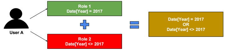
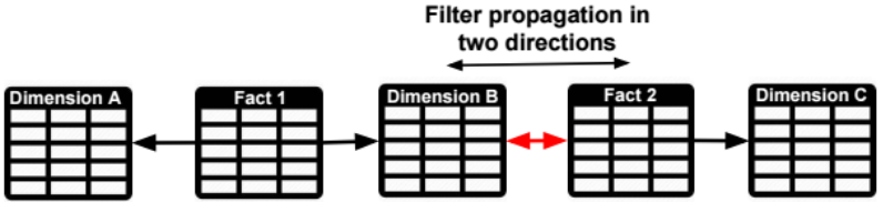
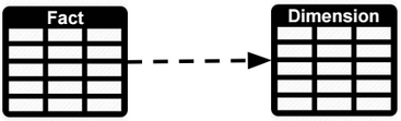
Role filters propagate through relationships (from the one side to the many side of one-to-many relationships).
To propagate role filters from the many side to the one side of a one-to-many relationship, we need to set filter direction to “Both Tables”, and check the checkbox “Apply the Filter Direction when using row Level Security”. 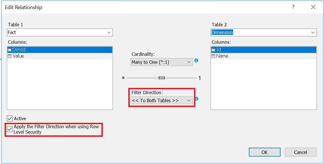
Role filters cannot be applied on calculated columns when a Tabular model is In-Memory mode, because calculated columns are evaluated during model processing. In Direct Query mode, role filters are applied when querying source tables.
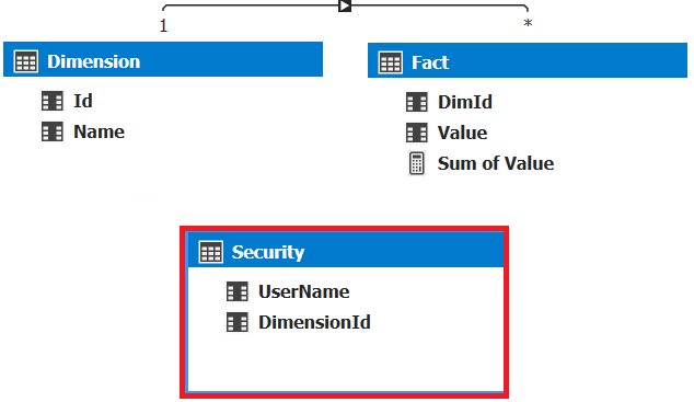
Dynamic Security
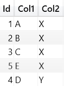
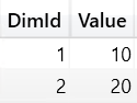
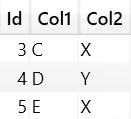
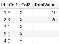
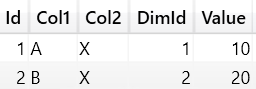
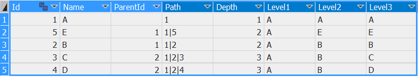
In the following Tabular model, we use the table “Security” to filter Fact table rows. The DAX filter expression is highlighted in red in the following image.
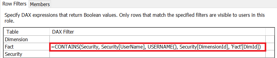
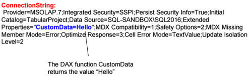
We can filter rows using an external parameter defined in the connection string. We can read the value of this parameter using the DAX function CUSTOMDATA.
Deployment
There are 4 ways to deploy a tabular model:
1-Using XMLA/TMSL
2-Using SSAS Deployment Wizard
3-Using Synchronize Wizard (Source and destination servers cannot be the same. In general, Synchronize is used to move a database from processing server to main server)
4-Backup/Restore database
.Net libraries
There are two libraries: Analysis Management Objects (AMO) and Tabular Object Model (TOM) that we can use to interact with the SSAS server.
Recommandations
Avoid large dimensions containing more than one million rows.
More articles and courses related to SSAS Tabular, Power BI and DAX can be found in the SQLBI website: http://www.sqlbi.com/.