A Tensor is a multidimensional array.
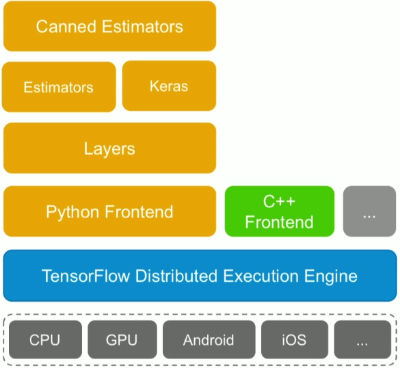
TensorFlow uses static computational graphs to train models. Dynamic computational graphs are more complicated to define using TensorFlow.
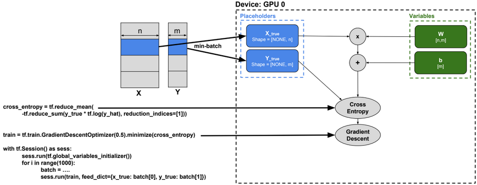
Multiclass classification
Below the execution steps of a TensorFlow code for multiclass classification:
1-Select a device (GPU or CPU)
2-Initialize a session
3-Initialize variables
4-Use mini-batches and run multiple SGD training steps
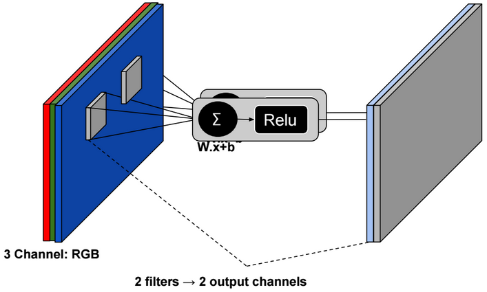
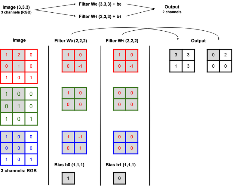
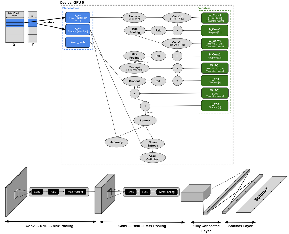
Convolutional Neural Network
Below a TensorFlow code for a Convolutional Neural Network.
import tensorflow as tf
from tensorflow.examples.tutorials.mnist import input_data
mnist = input_data.read_data_sets(‘MNIST_data’, one_hot=True)
width, height = 28, 28
flat = width * height
class_output = 10
x_true = tf.placeholder(tf.float32, shape=[None, flat])
y_true = tf.placeholder(tf.float32, shape=[None, class_output])
x_image = tf.reshape(x_true, [-1,28,28,1])
W_conv1 = tf.Variable(tf.truncated_normal([5, 5, 1, 32], stddev=0.1))
b_conv1 = tf.Variable(tf.constant(0.1, shape=[32]))
convolve1= tf.nn.conv2d(x_image, W_conv1, strides=[1, 1, 1, 1], padding=’SAME’) + b_conv1
h_conv1 = tf.nn.relu(convolve1)
conv1 = tf.nn.max_pool(h_conv1, ksize=[1, 2, 2, 1], strides=[1, 2, 2, 1], padding=’SAME’)
W_conv2 = tf.Variable(tf.truncated_normal([5, 5, 32, 64], stddev=0.1))
b_conv2 = tf.Variable(tf.constant(0.1, shape=[64]))
convolve2= tf.nn.conv2d(conv1, W_conv2, strides=[1, 1, 1, 1], padding=’SAME’)+ b_conv2
h_conv2 = tf.nn.relu(convolve2)
conv2 = tf.nn.max_pool(h_conv2, ksize=[1, 2, 2, 1], strides=[1, 2, 2, 1], padding=’SAME’)
layer2_matrix = tf.reshape(conv2, [-1, 7*7*64])
W_fc1 = tf.Variable(tf.truncated_normal([7 * 7 * 64, 1024], stddev=0.1))
b_fc1 = tf.Variable(tf.constant(0.1, shape=[1024]))
fcl=tf.matmul(layer2_matrix, W_fc1) + b_fc1
h_fc1 = tf.nn.relu(fcl)
keep_prob = tf.placeholder(tf.float32)
layer_drop = tf.nn.dropout(h_fc1, keep_prob)
W_fc2 = tf.Variable(tf.truncated_normal([1024, 10], stddev=0.1))
b_fc2 = tf.Variable(tf.constant(0.1, shape=[10])) # 10 possibilities for digits [0,1,2,3,4,5,6,7,8,9]
fc=tf.matmul(layer_drop, W_fc2) + b_fc2
y_CNN= tf.nn.softmax(fc)
cross_entropy = tf.reduce_mean(-tf.reduce_sum(y_true * tf.log(y_CNN), reduction_indices=[1]))
train_step = tf.train.AdamOptimizer(1e-4).minimize(cross_entropy)
correct_prediction = tf.equal(tf.argmax(y_CNN,1), tf.argmax(y_true,1))
accuracy = tf.reduce_mean(tf.cast(correct_prediction, tf.float32))
sess = tf.InteractiveSession()
sess.run(tf.global_variables_initializer())
for i in range(2000):
batch = mnist.train.next_batch(50)
if i%100 == 0:
train_accuracy = sess.run(accuracy, feed_dict={
x_true:batch[0], y_true: batch[1], keep_prob: 1.0})
print(“step %d, training accuracy %g”%(i, train_accuracy))
sess.run(train_step, feed_dict={x_true: batch[0], y_true: batch[1], keep_prob: 0.5})
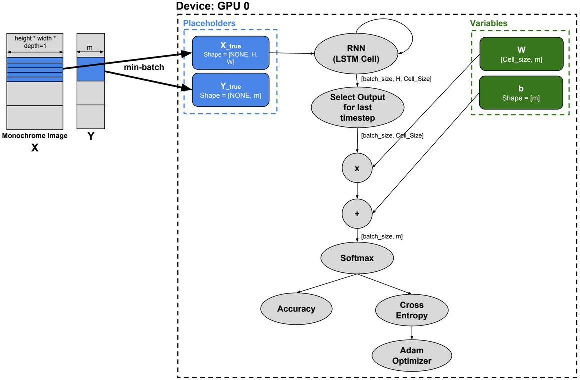
Image Classification using LSTM
Image rows are used as sequences to train the RNN model.
import tensorflow as tf
from tensorflow.examples.tutorials.mnist import input_data
mnist = input_data.read_data_sets(“.”, one_hot=True)
n_input = 28 # MNIST data input (img shape: 28*28)
n_steps = 28 # timesteps
n_hidden = 128 # hidden layer num of features
n_classes = 10 # MNIST total classes (0-9 digits)
# Current data input shape: (batch_size, n_steps, n_input) [100x28x28]
x_true = tf.placeholder(dtype=”float”, shape=[None, n_steps, n_input], name=”x”)
y_true = tf.placeholder(dtype=”float”, shape=[None, n_classes], name=”y”)
lstm_cell = tf.contrib.rnn.BasicLSTMCell(n_hidden, forget_bias=1.0)
#dynamic_rnn creates a recurrent neural network specified from lstm_cell
#The output of the rnn would be a [batch_size x n_steps x n_hidden] matrix
outputs, states = tf.nn.dynamic_rnn(lstm_cell, inputs=x_true, dtype=tf.float32)
learning_rate = 0.001
training_iters = 100000
batch_size = 100
display_step = 10
W = tf.Variable(tf.random_normal([n_hidden, n_classes]))
b = tf.Variable(tf.random_normal([n_classes]))
output = tf.reshape(tf.split(outputs, 28, axis=1, num=None, name=’split’)[-1],[-1,128])
pred = tf.matmul(output, W) + b
cost = tf.reduce_mean(tf.nn.softmax_cross_entropy_with_logits(labels=y_true, logits=pred))
optimizer = tf.train.AdamOptimizer(learning_rate=learning_rate).minimize(cost)
correct_pred = tf.equal(tf.argmax(pred,1), tf.argmax(y_true,1))
accuracy = tf.reduce_mean(tf.cast(correct_pred, tf.float32))
init = tf.global_variables_initializer()
with tf.Session() as sess:
sess.run(init)
step = 1
# Keep training until reach max iterations
while step * batch_size < training_iters:
# We will read a batch of 100 images [100 x 784] as batch_x
# batch_y is a matrix of [100×10]
batch_x, batch_y = mnist.train.next_batch(batch_size)
# We consider each row of the image as one sequence
# Reshape data to get 28 seq of 28 elements, so that, batch_x is [100x28x28]
batch_x = batch_x.reshape((batch_size, n_steps, n_input))
# Run optimization op (backprop)
sess.run(optimizer, feed_dict={x_true: batch_x, y_true: batch_y})
if step % display_step == 0:
# Calculate batch accuracy
acc = sess.run(accuracy, feed_dict={x_true: batch_x, y_true: batch_y})
# Calculate batch loss
loss = sess.run(cost, feed_dict={x_true: batch_x, y_true: batch_y})
print(“Iter ” + str(step*batch_size) + “, Minibatch Loss= ” + \
“{:.6f}”.format(loss) + “, Training Accuracy= ” + \
“{:.5f}”.format(acc))
step += 1
print(“Optimization Finished!”)
# Calculate accuracy for 128 mnist test images
test_len = 128
test_data = mnist.test.images[:test_len].reshape((-1, n_steps, n_input))
test_label = mnist.test.labels[:test_len]
print(“Testing Accuracy:”, \
sess.run(accuracy, feed_dict={x_true: test_data, y_true: test_label}))
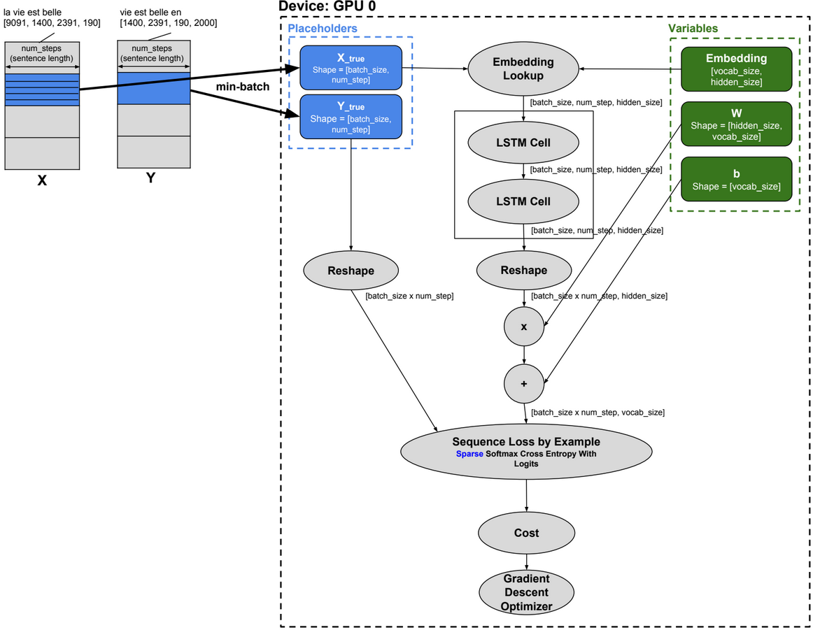
Language Modelling using LSTM
import time
import numpy as np
import tensorflow as tf
!wget -q -O /resources/data/ptb.zip https://ibm.box.com/shared/static/z2yvmhbskc45xd2a9a4kkn6hg4g4kj5r.zip
!unzip -o /resources/data/ptb.zip -d /resources/
!cp /resources/ptb/reader.py .
import reader
!wget http://www.fit.vutbr.cz/~imikolov/rnnlm/simple-examples.tgz
!tar xzf simple-examples.tgz -C /resources/data/
batch_size = 30
num_steps = 20
hidden_size = 200
num_layers = 2
vocab_size = 10000
data_dir = “/resources/data/simple-examples/data/”
# Reads the data and separates it into training data, validation data and testing data
raw_data = reader.ptb_raw_data(data_dir)
train_data, valid_data, test_data, _ = raw_data
_input_data = tf.placeholder(tf.int32, [batch_size, num_steps])
_targets = tf.placeholder(tf.int32, [batch_size, num_steps])
lstm_cell = tf.contrib.rnn.BasicLSTMCell(hidden_size, forget_bias=0.0)
stacked_lstm = tf.contrib.rnn.MultiRNNCell([lstm_cell] * num_layers)
embedding = tf.get_variable(“embedding”, [vocab_size, hidden_size])
inputs = tf.nn.embedding_lookup(embedding, _input_data)
outputs, new_state = tf.nn.dynamic_rnn(stacked_lstm, inputs, dtype=tf.float32)
output = tf.reshape(outputs, [-1, hidden_size])
softmax_w = tf.get_variable(“softmax_w”, [hidden_size, vocab_size]) #[200×1000]
softmax_b = tf.get_variable(“softmax_b”, [vocab_size]) #[1×1000]
logits = tf.matmul(output, softmax_w) + softmax_b
loss = tf.contrib.legacy_seq2seq.sequence_loss_by_example([logits], [tf.reshape(_targets, [-1])],[tf.ones([batch_size * num_steps])])
cost = tf.reduce_sum(loss) / batch_size
# Create a variable for the learning rate
lr = tf.Variable(0.0, trainable=False)
# Create the gradient descent optimizer with our learning rate
optimizer = tf.train.GradientDescentOptimizer(lr)
#Maximum permissible norm for the gradient (For gradient clipping — another measure against Exploding Gradients)
max_grad_norm = 5
tvars = tf.trainable_variables()
grad_t_list = tf.gradients(cost, tvars)
grads, _ = tf.clip_by_global_norm(grad_t_list, max_grad_norm)
train_op = optimizer.apply_gradients(zip(grads, tvars))
session=tf.InteractiveSession()
session.run(tf.global_variables_initializer())
itera = reader.ptb_iterator(train_data, batch_size, num_steps)
first_touple=itera.next()
x=first_touple[0]
y=first_touple[1]
session.run(train_op, feed_dict={_input_data:x, _targets:y})
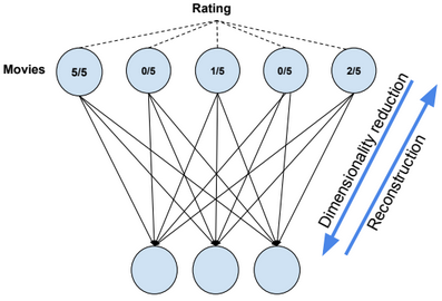
Collaborative Filtering with RBM
import tensorflow as tf
import numpy as np
import pandas as pd
import matplotlib.pyplot as plt
visibleUnits = 5
hiddenUnits = 3
vb = tf.placeholder(“float”, [visibleUnits]) #Number of unique movies
hb = tf.placeholder(“float”, [hiddenUnits]) #Number of features we’re going to learn
W = tf.placeholder(“float”, [visibleUnits, hiddenUnits])
#Phase 1: Input Processing
v0 = tf.placeholder(“float”, [None, visibleUnits])
_h0= tf.nn.sigmoid(tf.matmul(v0, W) + hb)
h0 = tf.nn.relu(tf.sign(_h0 – tf.random_uniform(tf.shape(_h0))))
#Phase 2: Reconstruction
_v1 = tf.nn.sigmoid(tf.matmul(h0, tf.transpose(W)) + vb)
v1 = tf.nn.relu(tf.sign(_v1 – tf.random_uniform(tf.shape(_v1))))
h1 = tf.nn.sigmoid(tf.matmul(v1, W) + hb)
#Learning rate
alpha = 1.0
#Create the gradients
w_pos_grad = tf.matmul(tf.transpose(v0), h0)
w_neg_grad = tf.matmul(tf.transpose(v1), h1)
#Calculate the Contrastive Divergence to maximize
CD = (w_pos_grad – w_neg_grad) / tf.to_float(tf.shape(v0)[0])
#Create methods to update the weights and biases
update_w = W + alpha * CD
update_vb = vb + alpha * tf.reduce_mean(v0 – v1, 0)
update_hb = hb + alpha * tf.reduce_mean(h0 – h1, 0)
err = v0 – v1
err_sum = tf.reduce_mean(err * err)
#Current weight
cur_w = np.zeros([visibleUnits, hiddenUnits], np.float32)
#Current visible unit biases
cur_vb = np.zeros([visibleUnits], np.float32)
#Current hidden unit biases
cur_hb = np.zeros([hiddenUnits], np.float32)
#Previous weight
prv_w = np.zeros([visibleUnits, hiddenUnits], np.float32)
#Previous visible unit biases
prv_vb = np.zeros([visibleUnits], np.float32)
#Previous hidden unit biases
prv_hb = np.zeros([hiddenUnits], np.float32)
sess = tf.Session()
sess.run(tf.global_variables_initializer())
epochs = 15
for i in range(epochs):
batch = [[.1,.5,.4,.4,.2], [.2,.0,.4,.1,.1], [.1,.0,.4,.1,.1],[.1,.1,.1,.1,.1]] #movies ratings
cur_w = sess.run(update_w, feed_dict={v0: batch, W: prv_w, vb: prv_vb, hb: prv_hb})
cur_vb = sess.run(update_vb, feed_dict={v0: batch, W: prv_w, vb: prv_vb, hb: prv_hb})
cur_nb = sess.run(update_hb, feed_dict={v0: batch, W: prv_w, vb: prv_vb, hb: prv_hb})
prv_w = cur_w
prv_vb = cur_vb
prv_hb = cur_nb
#Feeding in the user and reconstructing the input
hh0 = tf.nn.sigmoid(tf.matmul(v0, W) + hb)
vv1 = tf.nn.sigmoid(tf.matmul(hh0, tf.transpose(W)) + vb)
#Estimate user preferences for unwatched movies
feed = sess.run(hh0, feed_dict={ v0: [[.1,.1,.0,.0,.0]], W: prv_w, hb: prv_hb})
rec = sess.run(vv1, feed_dict={ hh0: feed, W: prv_w, vb: prv_vb})
print(rec)
Wrappers
Below some Tensorflow wrappers:
Keras, TFLearn, TensorLayer, Pretty Tensor, Sonnet.