This post describes some generative machine learning algorithms.

Gaussian Discriminant Analysis

Gaussian Discriminant Analysis is a supervised classification algorithm. In this algorithm we suppose the p(x|y) is multivariate Gaussian with parameter mean \(\overrightarrow{u}\) and covariance \(\Sigma : P(x|y) \sim N(\overrightarrow{u}, \Sigma) \).

If we suppose that y is Bernoulli distributed, then there are two distributions that can be defined, one for p(x|y=0) and one for p(x|y=1). The separator between these two distributions could be used to predict the values of y.

\(P(x|y=0) = \frac{1}{(2\pi)^{\frac{n}{2}}|\Sigma|^{\frac{1}{2}}} exp(-\frac{1}{2}(x – \mu_0)^T\Sigma^{-1}(x – \mu_0))\)

\(P(x|y=1) = \frac{1}{(2\pi)^{\frac{n}{2}}|\Sigma|^{\frac{1}{2}}} exp(-\frac{1}{2}(x – \mu_1)^T\Sigma^{-1}(x – \mu_1))\)

\(P(y) = \phi^y.(1-\phi)^{1-y}\)

We need to find \(\phi, \mu_0, \mu_1, \Sigma\) that maximize the log-likelihood function:

\(l(\phi, \mu_0, \mu_1, \Sigma) = log(\prod_{i=1}^{m} P(y^{(i)}|x^{(i)};\phi, \mu_0, \mu_1, \Sigma))\)

Using the Naive Bayes rule, we can transform the equation to:

\(= log(\prod_{i=1}^{m} P(x^{(i)} | y^{(i)};\mu_0, \mu_1, \Sigma) * P(y^{(i)};\phi))) – log(\prod_{i=1}^{m} P(x^{(i)}))\)

To maximize l, we need to maximize: \(log(\prod_{i=1}^{m} P(x^{(i)} | y^{(i)};\mu_0, \mu_1, \Sigma) * P(y^{(i)};\phi)))\)

For new data, to predict y, we need to calculate \(P(y=1|x) = \frac{P(x|y=1) * P(y=1)}{P(x|y=0)P(y=0) + P(x|y=1)P(y=1)}\) (P(y=0) and P(y=1) can be easily calculated from training data).

EM Algorithm

EM algorithm is an unsupervised clustering algorithm in which we assign a label to each training example. The clustering applied is soft clustering, which means that for each point we assign a probability for each label.

For a point x, we calculate the probability for each label.

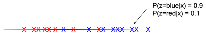
There are two main steps in this algorithm:

E-Step: Using the current estimate of parameters, calculate if points are more likely to come from the red distribution or the blue distribution.

M-Step: Re-estimate the parameters.

Given a training set \(S = \{x^{(i)}\}_{i=1}^m\). For each \(x^{(i)}\), there is hidden label \(z^{(i)}\) assigned to it.

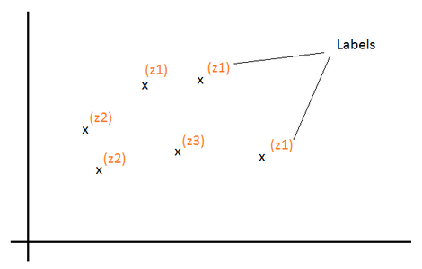
Z is a multinomial distribution with \(P(z = j)=?_j\).

k the number of distinct values of Z (number of classes).

For each \(x^{(i)}\), we would like to know the value \(z^{(i)}\) that is assigned to it. In other words, find \(l \in [1, k]\) that maximizes the probability \(P(z^{(i)} = l | x^{(i)})\)

Log-likelihood function to maximize: \(l(?) = log(\prod_{i=1}^m P(x^{(i)}; ?)) = \sum_{i=1}^m log(P(x^{(i)}; ?))\)

\( = \sum_{i=1}^m log(\sum_{l=1}^k P(x^{(i)}|z^{(i)} = l; ?) * P(z^{(i)} = l))\) \( = \sum_{i=1}^m log(\sum_{l=1}^k P(x^{(i)}, z^{(i)} = l; ?))\)

Let’s define \(Q_i\) as a probability distribution over Z: (\(Q_i(z^{(i)} = l)\) > = 0 and \(\sum_{l=1}^k Q_i(z^{(i)} = l) = 1\))

\(l(?) = \sum_{i=1}^m log(\sum_{l=1}^k Q_i(z^{(i)} = l) \frac{P(x^{(i)}, z^{(i)} = l; ?)}{Q_i(z^{(i)} = l)})\) \( = \sum_{i=1}^m log(E_{z^{(i)} \sim Q_i}[\frac{P(x^{(i)}, z^{(i)}; ?)}{Q_i(z^{(i)})}])\)

Log is concave function. Based on Jensen’s inequality log(E[X]) >= E[log(X)].

Then:

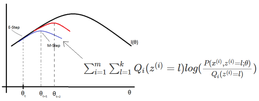
\(l(?) >= \sum_{i=1}^m E_{z^{(i)} \sim Q_i}[log(\frac{P(x^{(i)}, z^{(i)}; ?)}{Q_i(z^{(i)})})]\) \( = \sum_{i=1}^m \sum_{l=1}^k Q_i(z^{(i)}=l) log(\frac{P(x^{(i)}, z^{(i)}=l; ?)}{Q_i(z^{(i)}=l)})\)

If we set \(Q_i(z^{(i)}) = P(z^{(i)}| x^{(i)}; ?)\) then: \(\frac{P(x^{(i)}, z^{(i)}; ?)}{Q(z^{(i)})}\) \(= \frac{P(z^{(i)}| x^{(i)}; ?) * P(x^{(i)}; ?)}{P(z^{(i)}| x^{(i)}; ?)}\) \(= P(x^{(i)}; ?)\) = Constant (over z). In that case log(E[X]) = E[log(X)] and for the current estimate of ?, \(l(?) = \sum_{i=1}^m \sum_{l=1}^k Q_i(z^{(i)}=l) log(\frac{P(x^{(i)}, z^{(i)}=l; ?)}{Q_i(z^{(i)}=l)})\) (E-Step)

EM (Expectation-Maximization) algorithm for density estimation:

1-Initiliaze the parameters ?

2-For each i, set \(Q_i(z^{(i)}) = P(z^{(i)}| x^{(i)}; ?)\) (E-Step)

3-Update ? (M-Step)

\(? := arg\ \underset{?}{max} \sum_{i=1}^m \sum_{l=1}^k Q_i(z^{(i)}=l) log(\frac{P(x^{(i)}, z^{(i)}=l; ?)}{Q_i(z^{(i)}=l)})\)

Mixture of Gaussians

Given a value \(z^{(i)}=j\), If x is distributed normally \(N(?_j, ?_j)\), then:

\(Q_i(z^{(i)} = j) = P(z^{(i)} = j| x^{(i)}; ?)\) \(= \frac{P(x^{(i)} | z^{(i)}=j) * P(z^{(i)} = j)}{\sum_{l=1}^k P(x^{(i)} | z^{(i)}=l) * P(z^{(i)}=l)}\) \(= \frac{\frac{1}{{(2?)}^{\frac{n}{2}} |?_j|^\frac{1}{2}} exp(-\frac{1}{2} (x^{(i)}-?_j)^T {?_j}^{-1} (x^{(i)}-?_j)) * ?_j}{\sum_{l=1}^k \frac{1}{{(2?)}^{\frac{n}{2}} |?_l|^\frac{1}{2}} exp(-\frac{1}{2} (x^{(i)}-?_l)^T {?_l}^{-1} (x^{(i)}-?_l)) * ?_l}\)

Using the method of Lagrange Multipliers, we can find \(?_j, ?_j, ?_j\) that maximize: \(\sum_{i=1}^m \sum_{l=1}^k Q_i(z^{(i)}=l) log(\frac{\frac{1}{{(2?)}^{\frac{n}{2}} |?_j|^\frac{1}{2}} exp(-\frac{1}{2} (x^{(i)}-?_j)^T {?_j}^{-1} (x^{(i)}-?_j)) * ?_j}{Q_i(z^{(i)}=l)})\) with the constraint \(\sum_{j=1}^k ?_j = 1\). We also need to set to zero the partial derivatives with respect to \(?_j\) and \(?_j\) and solve the equations to find the new values of these parameters. Repeat the operations until convergence.

More details about the algorithm can be found here: https://www.youtube.com/watch?v=ZZGTuAkF-Hw

Naive Bayes Classifier

Naive Bayes classifier is a supervised classification algorithm. In this algorithm, we try to calculate P(y|x), but this probability can be calculated using the naive bayes rule:

P(y|x) = P(x|y).P(y)/P(x)

If x is the vector \([x_1,x_2,…,x_n]\), then:

\(P(x|y) = P(x_1,x_2,…,x_n|y) = P(x_1|y) P(x_2|y, x_1) ….P(x_n|y, x_{n-1},…,x_1)\) \(P(x) = P(x1,x2,…,x_n)\)

If we suppose that \(x_i\) are conditionally independent (Naive Bayes assumption), then:

\(P(x|y) = P(x_1|y) * P(x_2|y) * … * P(x_n|y)\) \(= \prod_{i=1}^n P(x_i|y)\) \(P(x) = \prod_{i=1}^n P(x_i)\)

If \(\exists\) i such as \(P(x_i|y)=0\), then P(x|y) = 0. To avoid that case we need to use Laplace Smoothing when calculating probabilities.

We suppose that \(x_i \in \{0,1\}\) (one-hot encoding: [1,0,1,…,0]) and y \(\in \{0,1\}\).

We define \(\phi_{i|y=1}, \phi_{i|y=0}, \phi_y\) such as:

\(P(x_i=1|y=1) = \phi_{i|y=1} \\ P(x_i=0|y=1) = 1 – \phi_{i|y=1}\) \(P(x_i=1|y=0) = \phi_{i|y=0} \\ P(x_i=0|y=0) = 1 – \phi_{i|y=0}\) \(P(y) = \phi_y^y.(1-\phi_y)^{1-y}\)

We need to find \(\phi_y, \phi_{i|y=0}, \phi_{i|y=1}\) that maximize the log-likelihood function:

\(l(\phi, \phi_{i|y=0}, \phi_{i|y=1}) = log(\prod_{i=1}^{m} \prod_{j=1}^n P(x_j^{(i)}|y^{(i)}) P(y^{(i)})/P(x^{(i)}))\)

Or maximize the following expression:

\(log(\prod_{i=1}^{m} \prod_{j=1}^n P(x_j^{(i)}|y^{(i)}) P(y^{(i)}))\)