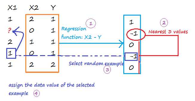
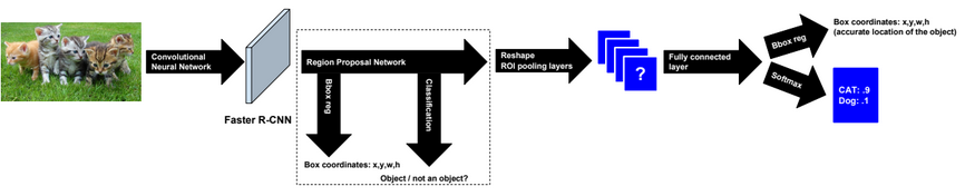
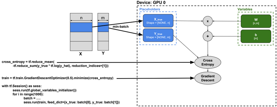
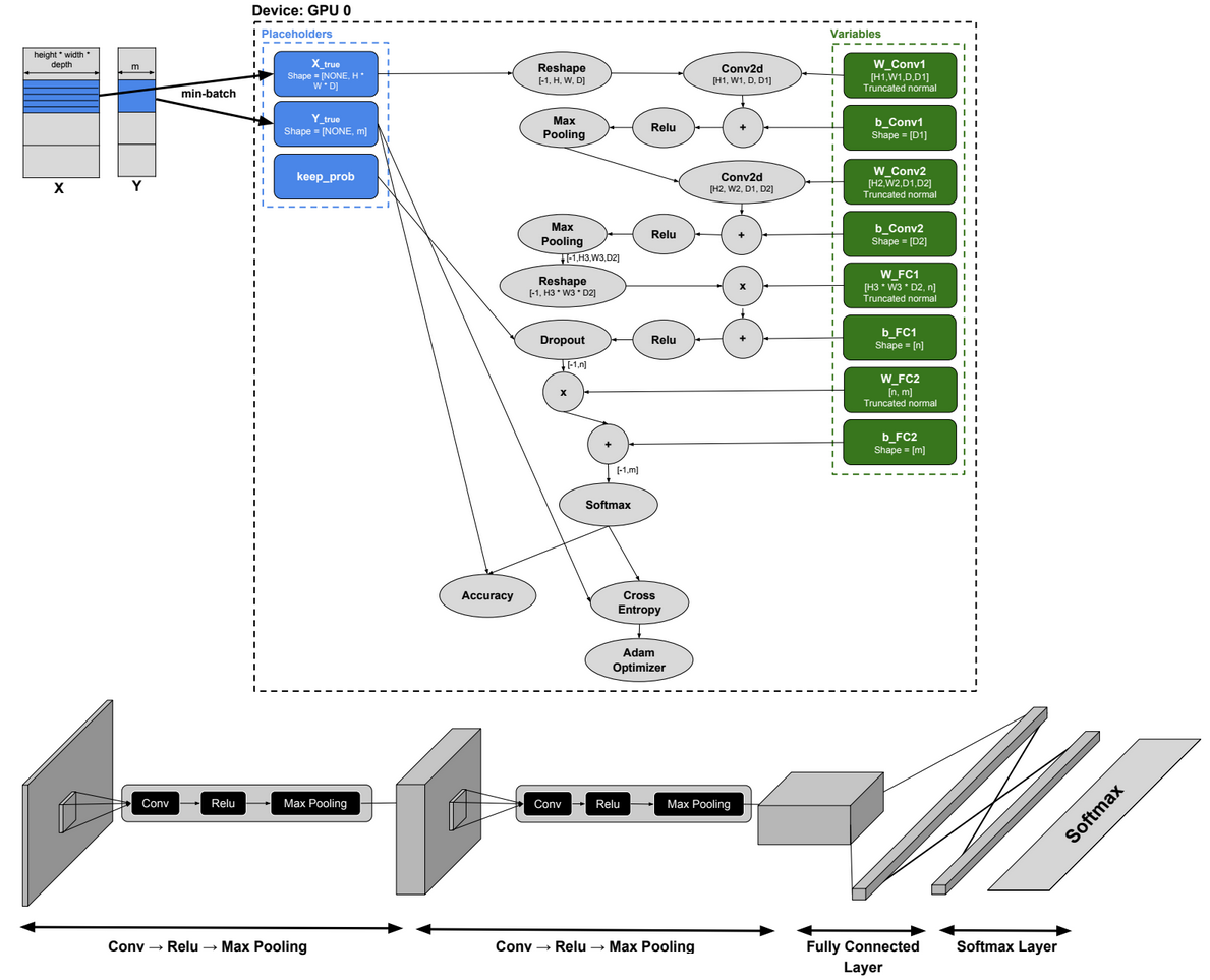
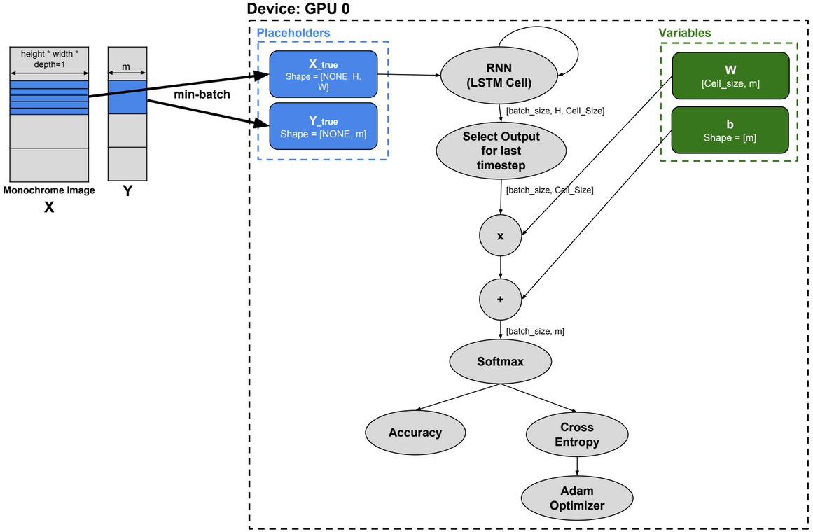
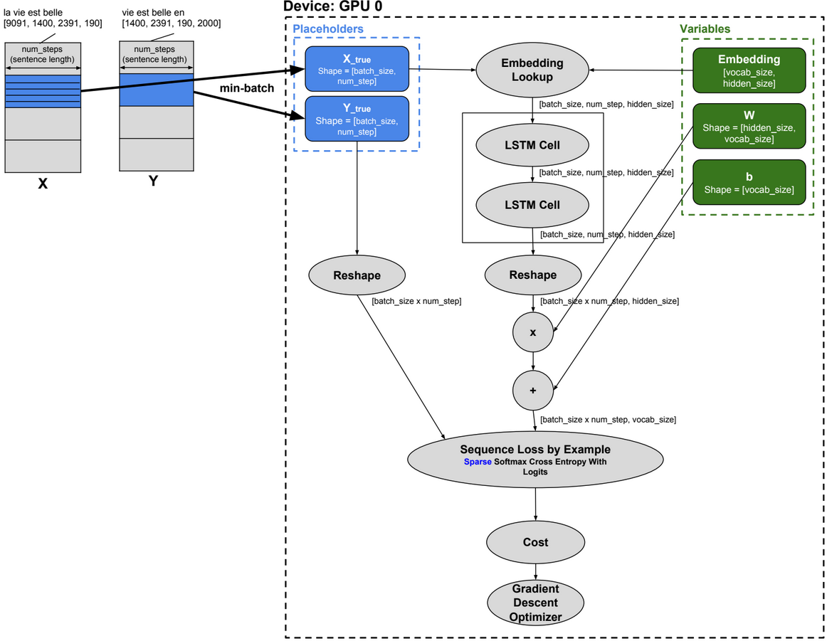
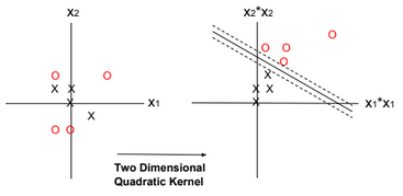
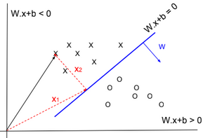
Dimensionality reduction is used to remove irrelevant and redundant features.

When the number of features in a dataset is bigger than the number of examples, then the probability density function of the dataset becomes difficult to calculate.

For example, if we model a dataset \(S = \{x^{(i)}\}_{i=1}^m,\ x \in R^{n}\) as a single Gaussian N(μ, ∑), then the probability density function is defined as: \(P(x) = \frac{1}{{(2Ï€)}^{\frac{n}{2}} |Σ|^\frac{1}{2}} exp(-\frac{1}{2} (x-μ)^T {Σ}^{-1} (x-μ))\) such as \(μ = \frac{1}{m} \sum_{i=1}^m x^{(i)} \\ ∑ = \frac{1}{m} \sum_{i=1}^m (x^{(i)} – μ)(x^{(i)} – μ)^T\).

But If n >> m, then ∑ will be singular, and calculating P(x) will be impossible.

Note: \((x^{(i)} – μ)(x^{(i)} – μ)^T\) is always singular, but the \(\sum_{i=1}^m\) of many singular matrices is most likely invertible when m >> n.

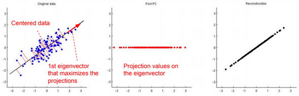
Principal Component Analysis

Given a set \(S = \{x^{(1)}=(0,1), x^{(2)}=(1,1)\}\), to reduce the dimensionality of S from 2 to 1, we need to project data on a vector that maximizes the projections. In other words, find the normalized vector \(μ = (μ_1, μ_2)\) that maximizes \( ({x^{(1)}}^T.μ)^2 + ({x^{(2)}}^T.μ)^2 = (μ_2)^2 + (μ_1 + μ_2)^2\).

Using the method of Lagrange Multipliers, we can solve the maximization problem with constraint \(||u|| = μ_1^2 + μ_2^2 = 1\).

\(L(μ, λ) = (μ_2)^2 + (μ_1 + μ_2)^2 – λ (μ_1^2 + μ_2^2 – 1) \)

We need to find μ such as \(∇_u = 0 \) and ||u|| = 1

After derivations we will find that the solution is the vector μ = (0.52, 0.85)

Generalization

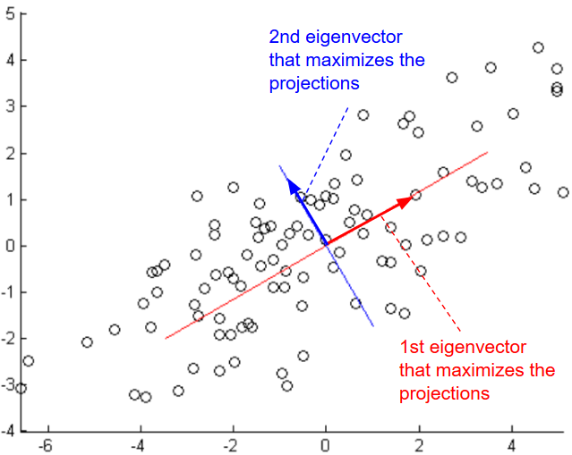
Given a set \(S = \{x^{(i)}\}_{i=1}^m,\ x \in R^{n}\), to reduce the dimensionality of S, we need to find μ that maximizes \(arg \ \underset{u: ||u|| = 1}{max} \frac{1}{m} \sum_{i=1}^m ({x^{(i)}}^T u)^2\)

\(=\frac{1}{m} \sum_{i=1}^m (u^T {x^{(i)}})({x^{(i)}}^T u)\) \(=u^T (\frac{1}{m} \sum_{i=1}^m {x^{(i)}} * {x^{(i)}}^T) u\)

Let’s define \( ∑ = \frac{1}{m} \sum_{i=1}^m {x^{(i)}} * {x^{(i)}}^T \)

Using the method of Lagrange Multipliers, we can solve the maximization problem with constraint \(||u|| = u^Tu\) = 1.

\(L(μ, λ) = u^T ∑ u – λ (u^Tu – 1) \)

If we calculate the derivative with respect to u, we will find:

\(∇_u = ∑ u – λ u = 0\)

Therefore u that solves this maximization problem must be an eigenvector of ∑. We need to choose the eigenvector with highest eigenvalue.

If we choose k eigenvectors \({u_1, u_2, …, u_k}\), then we need to transform the data by multiplying each example with each eigenvector.

\(x^{(i)} := (u_1^T x^{(i)}, u_2^T x^{(i)},…, , u_k^T x^{(i)}) = U^T x^{(i)}\)

Data should be normalized before running the PCA algorithm:

1-\(μ = \frac{1}{m} \sum_{i=1}^m x^{(i)}\)

2-\(x^{(i)} := x^{(i)} – μ\)

3-\(σ_j^{(i)} = \frac{1}{m} \sum_{i=1}^m {x_j^{(i)}}^2\)

4-\(x^{(i)} := \frac{x_j^{(i)}}{σ_j^{(i)}}\)

To reconstruct the original data, we need to calculate \(\widehat{x}^{(i)} := U^T x^{(i)}\)

Factor Analysis

Factor analysis is a way to take a mass of data and shrinking it to a smaller data set with less features.

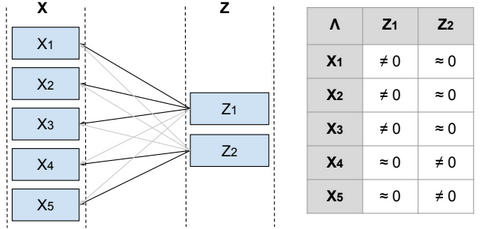
Given a set \(S = \{x^{(i)}\}_{i=1}^m,\ x \in R^{n}\), and S is modeled as a single Gaussian.

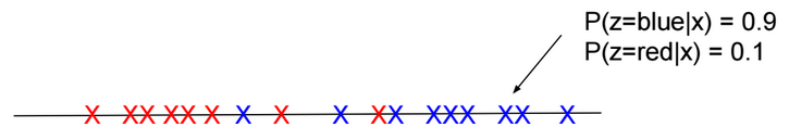
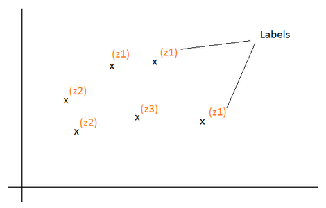
To reduce the dimensionality of S, we define a relationship between the variable x and a laten (hidden) variable z called factor such as \(x^{(i)} = μ + Λ z^{(i)} + ϵ^{(i)}\) and \(μ \in R^{n}\), \(z^{(i)} \in R^{d}\), \(Λ \in R^{n*d}\), \(ϵ \sim N(0, Ψ)\), Ψ is diagonal, \(z \sim N(0, I)\) and d <= n.

From Λ we can find the features that are related to each factor, and then identify the features that need to be eliminated or combined in order to reduce the dimensionality of the data.

Below the steps to estimate the parameters Ψ, μ, Λ.

\(E[x] = E[μ + Λz + ϵ] = E[μ] + ΛE[z] + E[ϵ] = μ \) \(Var(x) = E[(x – μ)^2] = E[(x – μ)(x – μ)^T] = E[(Λz + ϵ)(Λz + ϵ)^T]\) \(=E[Λzz^TΛ^T + ϵz^TΛ^T + Λzϵ^T + ϵϵ^T]\) \(=ΛE[zz^T]Λ^T + E[ϵz^TΛ^T] + E[Λzϵ^T] + E[ϵϵ^T]\) \(=Λ.Var(z).Λ^T + E[ϵz^TΛ^T] + E[Λzϵ^T] + Var(ϵ)\)

ϵ and z are independent, then the join probability of p(ϵ,z) = p(ϵ)*p(z), and \(E[ϵz]=\int_{ϵ}\int_{z} ϵ*z*p(ϵ,z) dϵ dz\)

\(=\int_{ϵ}\int_{z} ϵ*z*p(ϵ)*p(z) dϵ dz\) \(=\int_{ϵ} ϵ*p(ϵ) \int_{z} z*p(z) dz dϵ\) \(=E[ϵ]E[z]\)

So:

\(Var(x)=ΛΛ^T + Ψ\)

Therefore \(x \sim N(μ, ΛΛ^T + Ψ)\) and \(P(x) = \frac{1}{{(2π)}^{\frac{n}{2}} |ΛΛ^T + Ψ|^\frac{1}{2}} exp(-\frac{1}{2} (x-μ)^T {(ΛΛ^T + Ψ)}^{-1} (x-μ))\)

\(Λ \in R^{n*d}\), if d <= m, then \(ΛΛ^T + Ψ\) is most likely invertible.

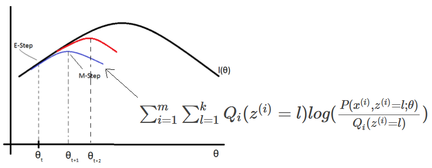
To find Ψ, μ, Λ, we need to maximize the log-likelihood function.

\(l(Ψ, μ, Λ) = \sum_{i=1}^m log(P(x^{(i)}; Ψ, μ, Λ))\) \(= \sum_{i=1}^m log(\frac{1}{{(2π)}^{\frac{n}{2}} |ΛΛ^T + Ψ|^\frac{1}{2}} exp(-\frac{1}{2} (x^{(i)}-μ)^T {(ΛΛ^T + Ψ)}^{-1} (x^{(i)}-μ)))\)

This maximization problem cannot be solved by calculating the \(∇_Ψ l(Ψ, μ, Λ) = 0\), \(∇_μ l(Ψ, μ, Λ) = 0\), \(∇_Λ l(Ψ, μ, Λ) = 0\). However using the EM algorithm, we can solve that problem.

More details can be found in this video: https://www.youtube.com/watch?v=ey2PE5xi9-A

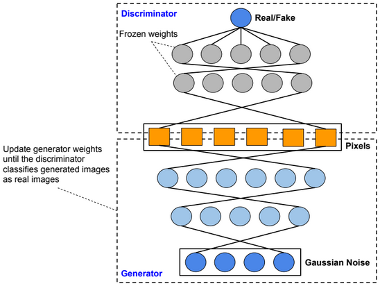
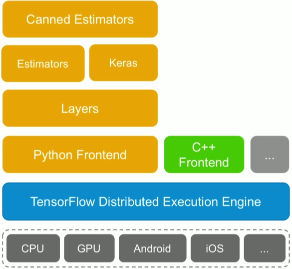
Restricted Boltzmann Machine

A restricted Boltzmann machine (RBM) is a two-layer stochastic neural network where the first layer consists of observed data variables (or visible units), and the second layer consists of latent variables (or hidden units). The visible layer is fully connected to the hidden layer. Both the visible and hidden layers are restricted to have no within-layer connections.

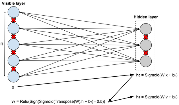
In this model, we update the parameters using the following equations:

\(W := W + α * \frac{x⊗Transpose(h_0) – v_1 ⊗ Transpose(h_1)}{n} \\ b_v := b_v + α * mean(x – v_1) \\ b_h := b_h + α * mean(h_0 – h_1) \\ error = mean(square(x – v_1))\).

Deep Belief Network

A deep belief network is obtained by stacking several RBMs on top of each other. The hidden layer of the RBM at layer i becomes the input of the RBM at layer i+1. The first layer RBM gets as input the input of the network, and the hidden layer of the last RBM represents the output.

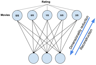
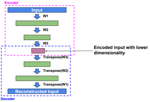
Autoencoders

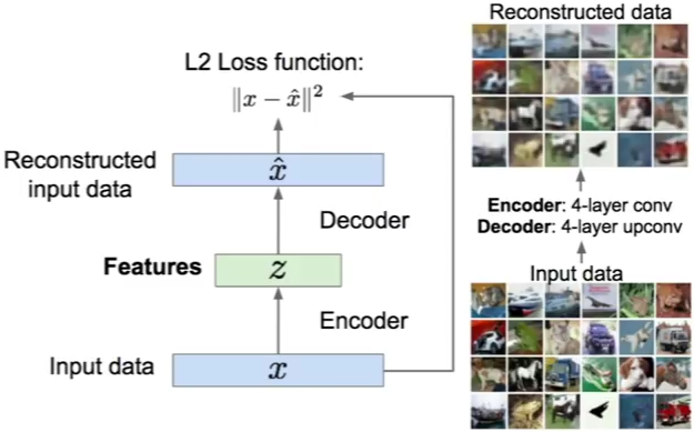
An autoencoder, autoassociator or Diabolo network is a deterministic artificial neural network used for unsupervised learning of efficient codings. The aim of an autoencoder is to learn a representation (encoding) for a set of data, typically for the purpose of dimensionality reduction. A deep Autoencoder contains multiple hidden units.

Loss function

For binary values, the loss function is defined as:

\(loss(x,\hat{x}) = -\sum_{k=1}^{size(x)} x_k.log(\hat{x_k}) + (1-x_k).log(1 – \hat{x_k})\).

For real values, the loss function is defined as:

\(loss(x,\hat{x}) = ½ \sum_{k=1}^{size(x)} (x_k – \hat{x_k})^2\).

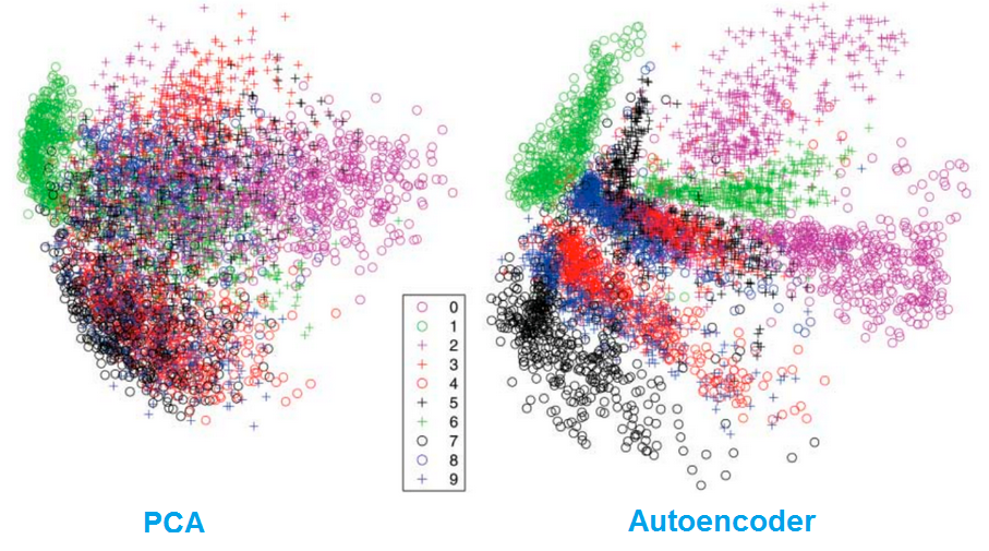
Dimensionality reduction

Autoencoders separate data better than PCA.

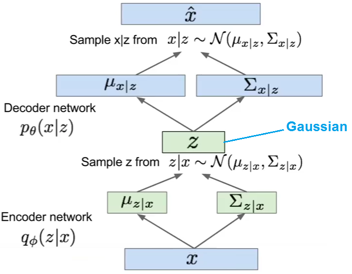
Variational Autoencoder

Variational autoencoder (VAE) models inherit autoencoder architecture, but make strong assumptions concerning the distribution of latent variables. In general, we suppose the distribution of the latent variable is gaussian.

The training algorithm used in VAEs is similar to EM algorithm.

Quantile Regression

Similar to Linear Regression, Quantile Regression estimates the conditional median instead of the conditional mean.

Decision Tree

Decision Tree is a classification algorithm.

Information Gain

Given the following training set {S}:

X1	X2	Y
a	c	e
a	d	e
b	d	f
b	d	f

We need to define the first level of the decision tree by choosing one of the two features x1 or x2. We need to calculate the Information Gain (I) for each case, and select the feature with higher Information Gain.

\(I(x) = Entropy(parent) – Expected Entropy(children) \) \(I(X1) = 1 – 0\) \(I(X2) = 1 – 0.688\)

When training the model, always use data with equal number of rows for each output, so the entropy of the root node equals to 1. (Entropy measure the uncertainty of the data).

Each node of the tree defines a probability estimation for each output.

More details: https://www.youtube.com/watch?v=-dCtJjlEEgM

Standard Deviation Reduction

Another approach to select features that define the levels of a decision tree is by calculating the Standard Deviation Reduction.

Boosted Decision Tree

A boosted decision tree is an ensemble learning method in which the second tree corrects for the errors of the first tree, the third tree corrects for the errors of the first and second trees, and so forth. The data points which were misclassified receives a bigger weight in the data, the ones correctly classified received a diminished weight. The idea is that with each iteration, the data points misclassified have increasing importance, allowing the learner to fit better and improve accuracy.

Predictions are based on the entire ensemble of trees together that makes the prediction.

Random Forest

When we have thousand of features (d), calculating the Information Gains for each split point and for each feature requires a lot of time and resources.

The idea in the Random Forest algorithm is to:

1-select a subset of size N from the training data

2-Pick up randomly k features, project the data on the k features, and select the split point with higher information gain.

Repeat step 2 until the creation of the tree (we can stop the operation at a certain depth of tree).

Repeat step 1 and 2 to generate more trees.

For a new example, we push it through all trees until it reaches the corresponding leaves. then we calculate the probability as the average of probabilities generated by all trees:

\(P(y=k|x) = \frac{1}{nbr\ trees} \sum_{t=1}^{nbr\ trees} P_t(y=k|x)\)

Clean Missing Data

How estimate missing data?

We can replace missing data with the Mean, the Median or the Mode, but usually it’s not an efficient approach.

If data are multi-variable distributed as below, if there is an example (x0, ?) with a missing value y, we can estimate y as a mean of values y for examples having x near to x0.

Linear regression based imputation

Find a model that estimates missing values based on other features: \(missing\_value = ?_0 + ?_1 * x_1 + ?_2 * x_2 + … + ?_{n+1} * y\)

MICE (Multiple Imputation through Chained Equations)

1-Replace all missing values with random values.

2-Pick randomly a value from one of the three nearest examples. The distance is calculated on values predicted using a regression function(linear, logistic, multinomial). Run the operation for each missing value.

Repeat step 1 and 2 m times to create m imputed data sets. Calculate the mean of imputed values from all imputed data sets, and assign it to each missing value of the original data set.

Probabilistic PCA

The PCA approach is based on the calcul of a low-dimensional approximation of the data, from which the full data is reconstructed. The new reconstructed matrix is used to fill missing values.

Filter based Feature Selection

Pearson Correlation

Pearson correlation coefficient:

\( r_{X,Y} = \frac{Cov(X,Y)}{?_X * ?_Y} \in [-1, 1]\)

Strong positive correlation when \(r_{X,Y}\) around 1.

No correlation when \(r_{X,Y}\) around 0.

Strong negative correlation when \(r_{X,Y}\) around -1.

Mutual Information

\(I(X,Y) = \sum_{x,y} p(x,y)*log(\frac{p(x,y)}{p(x)*p(y)}) >= 0\)

I(X,Y) = 0 when X, Y are independent

Kendall Correlation

Kendall correlation coefficient:

\(? = \frac{C-D}{C+D} \in [-1, 1]\)

C is the number of concordant pairs

D is the number of discordant pairs

X1 (Sorted)	X2	C	D
1	2	#values{X2>2 && X1>1}=3	#values{X2<2 && X1>1}=1
2	1	#values{X2>1 && X1>2}=3	#values{X2<1 && X1<2}=0
3	3	#values{X2>3 && X1>3}=2	#values{X2<3 && X1<3}=0
4	5	#values{X2>5 && X1>4}=0	#values{X2<5 && X1<4}=1
5	4	#values{X2>4 && X1>5}=0	#values{X2<4 && X1<5}=0
Total		8	2

\(? = \frac{C-D}{C+D} = 0.6\) (Good correlation)

For more details: https://www.youtube.com/watch?v=oXVxaSoY94k

Spearman Correlation

Spearman Correlation coefficient:

The Spearman correlation coefficient is defined as the Pearson correlation coefficient between the ranked variables.

\(r_S = \frac{Cov(rg\_X,rg\_Y)}{?_{rg\_X} * ?_{rg\_X}} \in [-1, 1]\)

X	Y	rg_X (X rank)	rg_Y (Y rank)
1	2	1	2
3	1	2	1
4	4	3	3
6	7	4	4
10	9	5	5

\(r_S = \frac{Cov(rg\_X,rg\_Y)}{?_{rg\_X} * ?_{rg\_Y}} = 0.8\)

Chi-Squared

Example:

X1	X2
1	2
3	1
3	1
3	1
3	2
3	2

Occurence X1/X2	1	2
1	0 (3/6)	1 (3/6)
2	0 (0/6)	0 (0/6)
3	3 (15/6)	2 (15/6)

In bold the expected value ((row total*column total)/n).

\(\chi^2 = \frac{(1-3/6)^2}{3/6} + \frac{(0-3/6)^2}{3/6} + \frac{(3-15/6)^2}{15/6} + \frac{(2-15/6)^2}{15/6}=1.2\)

Fisher Score

I don’t know the exact formula used, maybe the coefficient is calculated as below:

\( r = \frac{\sum_{i=1}^{n} (X_i – \overline{X})*(Y_i – \overline{Y})}{\sqrt{(\sum_{i=1}^{n} (X_i – \overline{X})^2) * (\sum_{i=1}^{n} (Y_i – \overline{Y})^2)}}\)

http://www.wikiwand.com/en/Fisher_transformation

Count-Based

Count of values for each feature.

Skewed Data

When training data are imbalanced (skewed), machine learning algorithms tend to minimize errors for the majority classes on the detriment of minority classes. It usually produces a biased classifier that has a higher predictive accuracy over the majority classes, but poorer predictive accuracy over the minority classes.

Synthetic Minority Oversampling Technique (SMOTE)

SMOTE is an algorithm that creates extra training data by performing certain operations on real data.

Given a set S = {(0,A), (1,A), (2,A), (3,A), (4,B), (5,B)}, A is the majority class, and B the minority class. If the amount of over-sampling needed is 200% (2x) and the number of nearest neighbors is 2, then the algorithm generates new samples in the following way:

Take the difference between an example under consideration and one of its nearest neighbor. Multiply this difference by a random number between 0 and 1, and add it to the feature vector under consideration.

Existing example (4,B) –> New example (4 + 0.3*(4-5), B)

Model Evaluation

Metrics

Mean Absolute Error	\(\frac{1}{m} \sum_{i=1}^{m} |y – h_?(x)|\)
Root Mean Squared Error (the standard deviation of the distribution of errors)	\(\sqrt{\frac{1}{m} \sum_{i=1}^{m} (y – h_?(x))^2} = \sqrt{J(?)}\)
Relative Absolute Error	\(\frac{\sum_{i=1}^{m} |y – h_?(x)|}{\sum_{i=1}^{m} |y – \frac{\sum_{i=1}^{m} y}{m}|}\)
Relative Squared Error	\(\frac{\sum_{i=1}^{m} (y – h_?(x))^2}{\sum_{i=1}^{m} (y – \frac{\sum_{i=1}^{m} y}{m})^2}\)
Coefficient of Determination (\(R^2\))	1 – [Relative Squared Error]

True Positive: \(1\{y=1, h_?(x)=1\}\)

False Positive: \(1\{y=0, h_?(x)=1\}\)

True Negative: \(1\{y=0, h_?(x)=0\}\)

False Negative:\(1\{y=1, h_?(x)=0\}\)

Accuracy	\(\frac{[True Positive] + [True Negative]}{m}\)
Precision	\(\frac{[True Positive]}{[True Positive] + [False Positive]}\)
Recall	\(\frac{[True Positive]}{[True Positive] + [True Negative]}\)
F1 Score	\(2 \frac{[Precision]*[Recall]}{[Precision]+[Recall]}\)

ROC Curve

Specificity: True Negative / (True Negative + False Positive)

Sensitivity: True Positive / (True Positive + False Negative)

AzureML components

Data Format Conversions

Convert to Dataset

Data Input/Output

Enter Data Manually
Import Data	Import from: Azure Block Storage, Azure SQL Database, Azure Table, Hive Query, Web URL, Data Feed Provider(OData), Azure DocumentDB
Export Data

Data Transformation

Edit Metadata	Rename columns
Join Data
Select Columns in Dataset
Remove Duplicate Rows
Slit Data
Partition and Sample	Select Top xxx rows, or generate a sample, or split data in k folds
Group Data into Bins
Clip Value	Remove outliers (peak and subpeak)
Build Counting Transform	For each selected column, and for an output class, calculate the occurrence of a value in all rows. Example: Country Product Advertised (2 classes) Country Class 0 Count Country Class 1 Count Product Class 0 Count Product Class 1 Count FR P1 0 1 0 2 1 CA P1 0 1 2 2 1 CA P1 1 1 2 2 1 CA P2 1 1 2 0 1 Note: On AzureML, we get wrong results if the number of rows is low.

Statistical Functions

Summarize Data

Machine Learning

Train Model
Tune Model Hyperparameters	Find best hyperparameter values
Score Model
Evaluate Model	Evaluate and compare one or two scored datasets
Train Clustering Model

R/Python Language Modules

Create R Model
Execute R Script
Execute Python Script	Supported Python packages: NumPy, pandas, SciPy, scikit-learn, matplotlib

Machine Learning Methods

Anomaly Detection Algorithms

One-Class SVM	The algorithm finds a minimal hypersphere around the data. Any point outside the hypersphere is considered an outlier.
PCA-Based Anomaly Detection	The algorithm applies PCA to reduce the dimensionality of the data, and applying distance metrics to identify cases that represent anomalies.

Classification Algorithms

Logistic Regression
Neural Network
Averaged Perceptron	Averaged Perceptron algorithm is an extension of the standard Perceptron algorithm; it uses averaged weights and biases.
Bayes Point Machine	It’s Bayesian linear classifier, therefore the model is not prone to overfitting
Decision Forest
Decision Jungle
Boosted Decision Tree
Decision Forest
Decision Jungle
SVM	The algorithm finds an optimal hyperplane that categorizes new examples. I didn’t know which kernel function is used by the algorithm. Probably it uses a linear kernel \(K(x,x’) = x^T .x’)\) SVM is not recommended with large training sets, because the classification of new examples requires the computation of kernels using all training examples.
Locally Deep SVM	The algorithm defines a tree to cluster examples (like Decision Tree algorithm), and then trains SVM on each cluster.
One-vs-All Multiclass	The One-vs-All Multiclass requires as an input multiple two-class classification algorithms. To classify a new example, the algorithm runs two-class classification algorithms for each class, then select the class with higher probability.

Clustering Algorithms

K-Means Clustering

Regression Algorithms

Bayesian Linear Regression	This model is not prone to overfitting
Boosted Decision Tree Regression
Decision Forest Regression
Fast Forest Quantile Regression
Neural Network Regression	Neural network with an output layer having no logistic function
Linear Regression
Ordinal Regression	Algorithm used for predicting an ordinal variable.
Poisson Regression	Algorithm used for predicting a Poisson variable

This post describes some geometric machine learning algorithms.

K-Nearest Neighbor Regression

k-nearest neighbors regression algorithm (k-NN regression) is a non-parametric method used for regression. For a new example x, predict y as the average of values \(y_1, y_2, …, y_k\) of k nearest neighbors of x.

K-Nearest Neighbor Classifier

k-nearest neighbors classifier (k-NN classifier) is a non-parametric method used for classification. For a new example x, predict y as the most common class among the k nearest neighbors of x.

Support Vector Machine (SVM)

In SVM, y has two values -1 or 1, and the hypothesis function is \(h_{W,b}(x) = g(W^T x + b)\) with g(z) = {1 if z >= 0, otherwise -1}.

We need to find W and b so \(W^T x + b\) >> 0 when y=1 and \(W^T x + b\) << 0 when y=-1

Functional margin

\(\widehat{?}^{(i)} = y^{(i)} . (W^T x^{(i)} +b)\)

We want that this function be >> 0 for all values of x.

We define \(\widehat{?} = min \ \widehat{?}^{(i)}\) for all values of i

Geometric margin

Geometric margin \(?^{(i)}\) is the geometric distance between an example \(x^{(i)}\) and the line defined by \(W^Tx + b = 0\). We define \(x_p^{(i)}\) as the point of projection of \(x^{(i)}\) on the line.

The vector \(\overrightarrow{x}^{(i)} = \overrightarrow{x_p}^{(i)} + ?^{(i)} * \frac{\overrightarrow{W}}{||W||} \)

\(x_p^{(i)}\) is in the line, then \(W^T (x^{(i)} – ?^{(i)} * \frac{W}{||W||}) + b = 0\)

We can find that \(?^{(i)} = \frac{W^T x^{(i)} + b}{||W||} \)

More generally \(?^{(i)} = y^{(i)}(\frac{W^T x^{(i)}}{||W||} + \frac{b}{||W||}) \)

We define \(? = min {?}^{(i)}\) for all values of i

We can deduce that the Geometric margin(?) = Functional margin / ||W||

Max Margin Classifier

We need to maximize the geometric margin \(?\), in other words \(\underset{W, b, ?}{max}\) ?, such as \(y^{(i)}(\frac{W^T x^{(i)}}{||W||} + \frac{b}{||W||})\) >= ? for all values \((x^{(i)},y^{(i)})\).

To simplify the maximization problem, we impose a scaling constraint: \(\widehat{?} = ? * ||W|| = 1\).

The optimization problem becomes as follow: \(\underset{W, b}{max}\frac{1}{||W||}\) (or \(\underset{W, b}{min}\frac{1}{2}||W||^2\)), such as \(y^{(i)}(W^T x^{(i)} + b)\) >= 1 for all values \((x^{(i)},y^{(j)})\).

Using the method of Lagrange Multipliers, we can solve the minimization problem.

\(L(W, b, ?) = \frac{1}{2} ||W||^2 – \sum_{i=1}^m ?_i * (y^{(i)}(W^T x^{(i)} + b) – 1)\)

Based on the KKT conditions, \(?_i >= 0\) and \(?_i * (y^{(i)}(W^T x^{(i)} + b) – 1) = 0\) for all i.

We know that \(y^{(i)}(W^T x^{(i)} + b) – 1 = 0\) is true only for few examples (called support vectors) located close to the the line \(W^Tx + b = 0\) (for these examples, \(? = {?}^{(i)} = \frac{1}{||W||}\)), therefore \(?_i\) is equal to 0 for the majority of examples.

By deriving L, we can find:

\(\frac{\partial L(W, b, ?)}{\partial w} = W – \sum_{i=1}^m ?_i * y^{(i)} * x^{(i)} = 0 \\ \frac{\partial L(W, b, ?)}{\partial b} = \sum_{i=1}^m ?_i * y^{(i)} = 0\)

After multiple derivations, we can find the equations for W, b and ?.

More details can be found in this video: https://www.youtube.com/watch?v=s8B4A5ubw6c

Predictions

The hypothesis function is defined as: \(h_{W,b}(x) = g(W^T x + b) = g(\sum_{i=1}^m ?_i * y^{(i)} * K(x^{(i)}, x) + b) \)

The function \(K(x^{(i)}, x) = ?(x^{(i)})^T ?(x) \) is known as the kernel function (? is a mapping function).

When ?(x) = x, then \(h_{W,b}(x) = g(\sum_{i=1}^m ?_i * y^{(i)} * (x^{(i)})^T . x + b) \)

Kernels

There are many types of kernels: “Polynomial kernel”, “Gaussian kernel”,…

In the example below the kernel is defined as Quadratic Kernel. \(K(x^{(i)}, x) = ?(x^{(i)})^T ?(x)\) and \(?(x) = (x_1^2, x_2^2, \sqrt{2} x_1 x_2)\). By using this kernel, SVM can find a linear separator (or hyperplane).

Regularization

Regularization can be applied to SVM by adding an extra term to the minimization function. The extra term relaxes the constraints by introducing slack variables. C is the regularization parameter.

\(\underset{W, b, ?_i}{min}\frac{||W||^2}{2} \color{red} {+ C \sum_{i=1}^m ?_i }\), such as \(y^{(i)}(W^T x^{(i)} + b)\) >= 1 – ?i for all values \((x^{(i)},y^{(j)})\) and \(?_i >= 0\).

The regularization parameter serves as a degree of importance that is given to miss-classifications. SVM poses a quadratic optimization problem that looks for maximizing the margin between both classes and minimizing the amount of miss-classifications. However, for non-separable problems, in order to find a solution, the miss-classification constraint must be relaxed.

As C grows larger, wrongly classified examples are not allowed, and when C tends to zero the more miss-classifications are allowed.

One-Class SVM

One-Class SVM is used to detect outliers. It finds a minimal hypersphere around the data. In other words, we need to minimize the radius R.

The minimization function for this model is defined as follow:

\(\underset{R, a, ?_i}{min} ||R||^2 + C \sum_{i=1}^m ?_i \), such as \(||x^{(i)} – a||^2 \leq R^2 + ?i\) for all values \((x^{(i)},y^{(j)})\) and \(?_i >= 0\).

Perceptron Algorithm

Similar to SVM, the Perceptron algorithm tries to separate positive and negative examples. There is no notion of kernel or margin maximization when using the perceptron algorithm. The algorithm can be trained online.

Averaged Perceptron Algorithm

Averaged Perceptron Algorithm is an extension of the standard Perceptron algorithm; it uses averaged weights and biases.

The classification of a new example is calculated by evaluating the following expression:

\(? = sign(\sum_{i=1}^m c_i.w_i^T.x + b_i)\)

Note: the sign of wx+b is related to the location of the point x.

w.x+b = w(x1+x2)+b = w.x2 because x1 is located on the blue line then w.x1+b = 0.

w.x2 is positive if the two vectors have the same direction.

K-means

Given a training set \(S = \{x^{(i)}\}_{i=1}^m\). We define k as the number of clusters (groups) to create. Each cluster has a centroid \(\mu_k\).

1-For each example, find j that minimizes: \(c^{(i)} := arg\ \underset{j}{min} ||x^{(i)} – \mu_j||^2\)

2-Update \(\mu_j:=\frac{\sum_{i=1}^m 1\{c^{(i)} = j\} x^{(i)}}{\sum_{i=1}^m 1\{c^{(i)} = j\}}\)

Repeat the operations 1 & 2 until convergence.

Large/Small Neural Networks

For a large amount of training data, use large networks.

Applying Machine Learning

Below the steps to apply machine learning to a business problem.

1-Collect DataSet

2-Prepare DataSet

3-Select & Design Model

4-Train Model

5-Evaluate Model

6-Test Model

Train/Dev/Test Sets

Training set: a set of examples used for training a ML model.

Dev (Validation or Cross-Validation) set: a set of examples used to tune hyper-parameters of a ML model.

Test set: a set of examples used to evaluate how well the model does with data outside the training/Dev set.

For deep learning algorithms, we no longer need to follow the common rules of (70%, 30%) ratios for Train and Test sets or (70%, 15%, 15%) ratios for Train, Dev and Test sets. Splitting data into 98% as training set and 2% as test set could be an acceptable option.

Error Analysis

Let us define first the following acronyms:

TP: True positive

FP: False positive

TN: True negative

FN: False negative

Accuracy	(TP + TN) / (TP + TN + FP + FN)
Precision	TP / (TP + FP)
Recall	TP / (TP + FN)
F1 score (best error metric)	2 (Precision * Recall) /(Precision + Recall)

Accuracy alone is a bad measure when data is skewed.

This post describes some generative machine learning algorithms.

Gaussian Discriminant Analysis

Gaussian Discriminant Analysis is a supervised classification algorithm. In this algorithm we suppose the p(x|y) is multivariate Gaussian with parameter mean \(\overrightarrow{u}\) and covariance \(\Sigma : P(x|y) \sim N(\overrightarrow{u}, \Sigma) \).

If we suppose that y is Bernoulli distributed, then there are two distributions that can be defined, one for p(x|y=0) and one for p(x|y=1). The separator between these two distributions could be used to predict the values of y.

\(P(x|y=0) = \frac{1}{(2\pi)^{\frac{n}{2}}|\Sigma|^{\frac{1}{2}}} exp(-\frac{1}{2}(x – \mu_0)^T\Sigma^{-1}(x – \mu_0))\)

\(P(x|y=1) = \frac{1}{(2\pi)^{\frac{n}{2}}|\Sigma|^{\frac{1}{2}}} exp(-\frac{1}{2}(x – \mu_1)^T\Sigma^{-1}(x – \mu_1))\)

\(P(y) = \phi^y.(1-\phi)^{1-y}\)

We need to find \(\phi, \mu_0, \mu_1, \Sigma\) that maximize the log-likelihood function:

\(l(\phi, \mu_0, \mu_1, \Sigma) = log(\prod_{i=1}^{m} P(y^{(i)}|x^{(i)};\phi, \mu_0, \mu_1, \Sigma))\)

Using the Naive Bayes rule, we can transform the equation to:

\(= log(\prod_{i=1}^{m} P(x^{(i)} | y^{(i)};\mu_0, \mu_1, \Sigma) * P(y^{(i)};\phi))) – log(\prod_{i=1}^{m} P(x^{(i)}))\)

To maximize l, we need to maximize: \(log(\prod_{i=1}^{m} P(x^{(i)} | y^{(i)};\mu_0, \mu_1, \Sigma) * P(y^{(i)};\phi)))\)

For new data, to predict y, we need to calculate \(P(y=1|x) = \frac{P(x|y=1) * P(y=1)}{P(x|y=0)P(y=0) + P(x|y=1)P(y=1)}\) (P(y=0) and P(y=1) can be easily calculated from training data).

EM Algorithm

EM algorithm is an unsupervised clustering algorithm in which we assign a label to each training example. The clustering applied is soft clustering, which means that for each point we assign a probability for each label.

For a point x, we calculate the probability for each label.

There are two main steps in this algorithm:

E-Step: Using the current estimate of parameters, calculate if points are more likely to come from the red distribution or the blue distribution.

M-Step: Re-estimate the parameters.

Given a training set \(S = \{x^{(i)}\}_{i=1}^m\). For each \(x^{(i)}\), there is hidden label \(z^{(i)}\) assigned to it.

Z is a multinomial distribution with \(P(z = j)=?_j\).

k the number of distinct values of Z (number of classes).

For each \(x^{(i)}\), we would like to know the value \(z^{(i)}\) that is assigned to it. In other words, find \(l \in [1, k]\) that maximizes the probability \(P(z^{(i)} = l | x^{(i)})\)

Log-likelihood function to maximize: \(l(?) = log(\prod_{i=1}^m P(x^{(i)}; ?)) = \sum_{i=1}^m log(P(x^{(i)}; ?))\)

\( = \sum_{i=1}^m log(\sum_{l=1}^k P(x^{(i)}|z^{(i)} = l; ?) * P(z^{(i)} = l))\) \( = \sum_{i=1}^m log(\sum_{l=1}^k P(x^{(i)}, z^{(i)} = l; ?))\)

Let’s define \(Q_i\) as a probability distribution over Z: (\(Q_i(z^{(i)} = l)\) > = 0 and \(\sum_{l=1}^k Q_i(z^{(i)} = l) = 1\))

\(l(?) = \sum_{i=1}^m log(\sum_{l=1}^k Q_i(z^{(i)} = l) \frac{P(x^{(i)}, z^{(i)} = l; ?)}{Q_i(z^{(i)} = l)})\) \( = \sum_{i=1}^m log(E_{z^{(i)} \sim Q_i}[\frac{P(x^{(i)}, z^{(i)}; ?)}{Q_i(z^{(i)})}])\)

Log is concave function. Based on Jensen’s inequality log(E[X]) >= E[log(X)].

Then:

\(l(?) >= \sum_{i=1}^m E_{z^{(i)} \sim Q_i}[log(\frac{P(x^{(i)}, z^{(i)}; ?)}{Q_i(z^{(i)})})]\) \( = \sum_{i=1}^m \sum_{l=1}^k Q_i(z^{(i)}=l) log(\frac{P(x^{(i)}, z^{(i)}=l; ?)}{Q_i(z^{(i)}=l)})\)

If we set \(Q_i(z^{(i)}) = P(z^{(i)}| x^{(i)}; ?)\) then: \(\frac{P(x^{(i)}, z^{(i)}; ?)}{Q(z^{(i)})}\) \(= \frac{P(z^{(i)}| x^{(i)}; ?) * P(x^{(i)}; ?)}{P(z^{(i)}| x^{(i)}; ?)}\) \(= P(x^{(i)}; ?)\) = Constant (over z). In that case log(E[X]) = E[log(X)] and for the current estimate of ?, \(l(?) = \sum_{i=1}^m \sum_{l=1}^k Q_i(z^{(i)}=l) log(\frac{P(x^{(i)}, z^{(i)}=l; ?)}{Q_i(z^{(i)}=l)})\) (E-Step)

EM (Expectation-Maximization) algorithm for density estimation:

1-Initiliaze the parameters ?

2-For each i, set \(Q_i(z^{(i)}) = P(z^{(i)}| x^{(i)}; ?)\) (E-Step)

3-Update ? (M-Step)

\(? := arg\ \underset{?}{max} \sum_{i=1}^m \sum_{l=1}^k Q_i(z^{(i)}=l) log(\frac{P(x^{(i)}, z^{(i)}=l; ?)}{Q_i(z^{(i)}=l)})\)

Mixture of Gaussians

Given a value \(z^{(i)}=j\), If x is distributed normally \(N(?_j, ?_j)\), then:

\(Q_i(z^{(i)} = j) = P(z^{(i)} = j| x^{(i)}; ?)\) \(= \frac{P(x^{(i)} | z^{(i)}=j) * P(z^{(i)} = j)}{\sum_{l=1}^k P(x^{(i)} | z^{(i)}=l) * P(z^{(i)}=l)}\) \(= \frac{\frac{1}{{(2?)}^{\frac{n}{2}} |?_j|^\frac{1}{2}} exp(-\frac{1}{2} (x^{(i)}-?_j)^T {?_j}^{-1} (x^{(i)}-?_j)) * ?_j}{\sum_{l=1}^k \frac{1}{{(2?)}^{\frac{n}{2}} |?_l|^\frac{1}{2}} exp(-\frac{1}{2} (x^{(i)}-?_l)^T {?_l}^{-1} (x^{(i)}-?_l)) * ?_l}\)

Using the method of Lagrange Multipliers, we can find \(?_j, ?_j, ?_j\) that maximize: \(\sum_{i=1}^m \sum_{l=1}^k Q_i(z^{(i)}=l) log(\frac{\frac{1}{{(2?)}^{\frac{n}{2}} |?_j|^\frac{1}{2}} exp(-\frac{1}{2} (x^{(i)}-?_j)^T {?_j}^{-1} (x^{(i)}-?_j)) * ?_j}{Q_i(z^{(i)}=l)})\) with the constraint \(\sum_{j=1}^k ?_j = 1\). We also need to set to zero the partial derivatives with respect to \(?_j\) and \(?_j\) and solve the equations to find the new values of these parameters. Repeat the operations until convergence.

More details about the algorithm can be found here: https://www.youtube.com/watch?v=ZZGTuAkF-Hw

Naive Bayes Classifier

Naive Bayes classifier is a supervised classification algorithm. In this algorithm, we try to calculate P(y|x), but this probability can be calculated using the naive bayes rule:

P(y|x) = P(x|y).P(y)/P(x)

If x is the vector \([x_1,x_2,…,x_n]\), then:

\(P(x|y) = P(x_1,x_2,…,x_n|y) = P(x_1|y) P(x_2|y, x_1) ….P(x_n|y, x_{n-1},…,x_1)\) \(P(x) = P(x1,x2,…,x_n)\)

If we suppose that \(x_i\) are conditionally independent (Naive Bayes assumption), then:

\(P(x|y) = P(x_1|y) * P(x_2|y) * … * P(x_n|y)\) \(= \prod_{i=1}^n P(x_i|y)\) \(P(x) = \prod_{i=1}^n P(x_i)\)

If \(\exists\) i such as \(P(x_i|y)=0\), then P(x|y) = 0. To avoid that case we need to use Laplace Smoothing when calculating probabilities.

We suppose that \(x_i \in \{0,1\}\) (one-hot encoding: [1,0,1,…,0]) and y \(\in \{0,1\}\).

We define \(\phi_{i|y=1}, \phi_{i|y=0}, \phi_y\) such as:

\(P(x_i=1|y=1) = \phi_{i|y=1} \\ P(x_i=0|y=1) = 1 – \phi_{i|y=1}\) \(P(x_i=1|y=0) = \phi_{i|y=0} \\ P(x_i=0|y=0) = 1 – \phi_{i|y=0}\) \(P(y) = \phi_y^y.(1-\phi_y)^{1-y}\)

We need to find \(\phi_y, \phi_{i|y=0}, \phi_{i|y=1}\) that maximize the log-likelihood function:

\(l(\phi, \phi_{i|y=0}, \phi_{i|y=1}) = log(\prod_{i=1}^{m} \prod_{j=1}^n P(x_j^{(i)}|y^{(i)}) P(y^{(i)})/P(x^{(i)}))\)

Or maximize the following expression:

\(log(\prod_{i=1}^{m} \prod_{j=1}^n P(x_j^{(i)}|y^{(i)}) P(y^{(i)}))\)