This post describes some discriminative machine learning algorithms.
|
Distribution of Y given X |
Algorithm to predict Y |
|
Normal distribution |
Linear regression |
|
Bernoulli distribution |
Logistic regression |
|
Multinomial distribution |
Multinomial logistic regression (Softmax regression) |
|
Exponential family distribution |
Generalized linear regression |
|
Distribution of X |
Algorithm to predict Y |
|
Multivariate normal distribution |
Gaussian discriminant analysis or EM Algorithm |
|
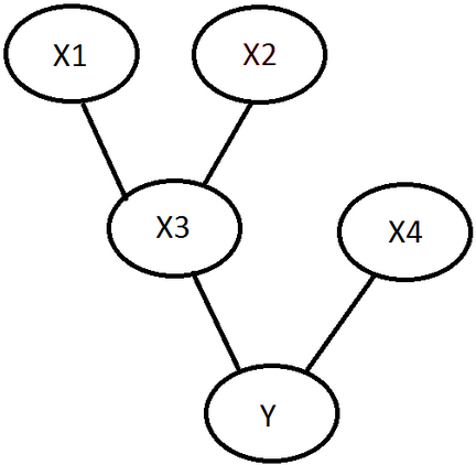
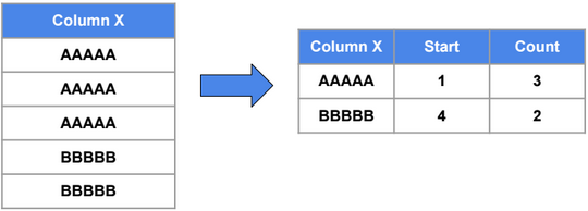
X Features conditionally independent \(p(x_1, x_2|y)=p(x_1|y) * p(x_2|y) \) |
Naive Bayes Algorithm |
Other ML algorithms are based on geometry, like the SVM and K-means algorithms.
Linear Regression
Below a table listing house prices by size.
|
x = House Size (\(m^2\)) |
y = House Price (k$) |
|
50 |
99 |
|
50 |
100 |
|
50 |
100 |
|
50 |
101 |
|
60 |
110 |
For the size 50\(m^2\), if we suppose that prices are normally distributed around the mean ╬╝=100 with a standard deviation Žā, then P(y|x = 50) = \(\frac{1}{\sigma \sqrt{2\pi}} exp(-\frac{1}{2} (\frac{y-╬╝}{\sigma})^{2})\)
We define h(x) as a function that returns the mean of the distribution of y given x (E[y|x]). We will define this function as a linear function. \(E[y|x] = h_{╬Ė}(x) = \theta^T x\)
P(y|x = 50; ╬Ė) = \(\frac{1}{\sigma \sqrt{2\pi}} exp(-\frac{1}{2} (\frac{y-h_{╬Ė}(x)}{\sigma})^{2})\)
We need to find ╬Ė that maximizes the probability for all values of x. In other words, we need to find ╬Ė that maximizes the likelihood function L:
\(L(\theta)=P(\overrightarrow{y}|X;╬Ė)=\prod_{i=1}^{n} P(y^{(i)}|x^{(i)};╬Ė)\)Or maximizes the log likelihood function l:
\(l(\theta)=log(L(\theta )) = \sum_{i=1}^{m} log(P(y^{(i)}|x^{(i)};\theta ))\) \(= \sum_{i=1}^{m} log(\frac{1}{\sigma \sqrt{2\pi}}) -\frac{1}{2} \sum_{i=1}^{n} (\frac{y^{(i)}-h_{╬Ė}(x^{(i)})}{\sigma})^{2}\)To maximize l, we need to minimize J(╬Ė) = \(\frac{1}{2} \sum_{i=1}^{m} (y^{(i)}-h_{╬Ė}(x^{(i)}))^{2}\). This function is called the Cost function (or Energy function, or Loss function, or Objective function) of a linear regression model. It’s also called “Least-squares cost function”.
J(╬Ė) is convex, to minimize it, we need to solve the equation \(\frac{\partial J(╬Ė)}{\partial ╬Ė} = 0\). A convex function has no local minimum.
There are many methods to solve this equation:
- Gradient descent (Batch or Stochastic Gradient descent)
- Normal equation
- Newton method
- Matrix differentiation
Gradient descent is the most used Optimizer (also called Learner or Solver) for learning model weights.
Batch Gradient descent
\(╬Ė_{j} := ╬Ė_{j} – \alpha \frac{\partial J(╬Ė)}{\partial ╬Ė_{j}} = ╬Ė_{j} – ╬▒ \frac{\partial \frac{1}{2} \sum_{i=1}^{n} (y^{(i)}-h_{╬Ė}(x^{(i)}))^{2}}{\partial ╬Ė_{j}}\)╬▒ is called “Learning rate”
\(╬Ė_{j} := ╬Ė_{j} – ╬▒ \frac{1}{2} \sum_{i=1}^{n} \frac{\partial (y^{(i)}-h_{╬Ė}(x^{(i)}))^{2}}{\partial ╬Ė_{j}}\)If \(h_{╬Ė}(x)\) is a linear function (\(h_{╬Ė} = ╬Ė^{T}x\)), then :
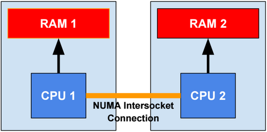
\(╬Ė_{j} := ╬Ė_{j} – ╬▒ \sum_{i=1}^{n} (h_{╬Ė}(x^{(i)}) – y^{(i)}) * x_j^{(i)} \)Batch size should fit the size of CPU or GPU memories, otherwise learning speed will be extremely slow.
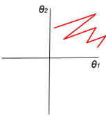
When using Batch gradient descent, the cost function in general decreases without oscillations.

Stochastic (Online) Gradient Descent (SGD) (use one example for each iteration – pass through all data N times (N Epoch))
\(╬Ė_{j} := ╬Ė_{j} – \alpha (h_{╬Ė}(x^{(i)}) – y^{(i)}) * x_j^{(i)} \)This learning rule is called “Least mean squares (LMS)” learning rule. It’s also called Widrow-Hoff learning rule.
Mini-batch Gradient descent
Run gradient descent for each mini-batch until we pass through traning set (1 epoch). Repeat the operation many times.
\(╬Ė_{j} := ╬Ė_{j} – \alpha \sum_{i=1}^{20} (h_{╬Ė}(x^{(i)}) – y^{(i)}) * x_j^{(i)} \)Mini-batch size should fit the size of CPU or GPU memories.
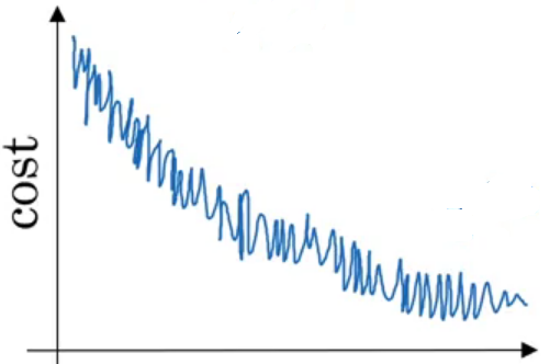
When using Batch gradient descent, the cost function decreases quickly but with oscillations.
Learning rate decay
ItŌĆÖs a technique used to automatically reduce learning rate after each epoch. Decay rate is a hyperparameter.
\(╬▒ = \frac{1}{1+ decayrate + epochnum} . ╬▒_0\)Momentum
Momentum is a method used to accelerate gradient descent. The idea is to add an extra term to the equation to accelerate descent steps.
\(╬Ė_{j_{t+1}} := ╬Ė_{j_t} – ╬▒ \frac{\partial J(╬Ė_{j_t})}{\partial ╬Ė_j} \color{blue} {+ ╬╗ (╬Ė_{j_t} – ╬Ė_{j_{t-1}})} \)Below another way to write the expression:
\(v(╬Ė_{j},t) = ╬▒ . \frac{\partial J(╬Ė_j)}{\partial ╬Ė_j} + ╬╗ . v(╬Ė_{j},t-1) \\ ╬Ė_{j} := ╬Ė_{j} – \color{blue} {v(╬Ė_{j},t)}\)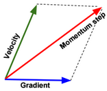
Nesterov Momentum is a slightly different version of momentum method.
AdaGrad
Adam is another method used to accelerate gradient descent.
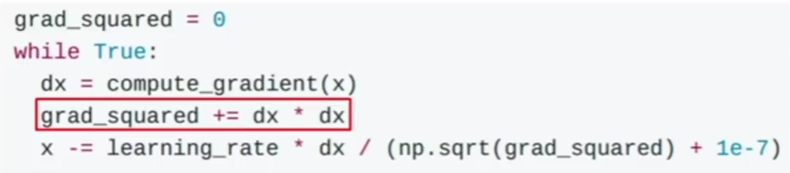
The problem in this method is that the term grad_squared becomes large after running many gradient descent steps. The term grad_squared is used to accelerate gradient descent when gradients are small, and slow down gradient descent when gradients are large.
RMSprop
RMSprop is an enhanced version of AdaGrad.
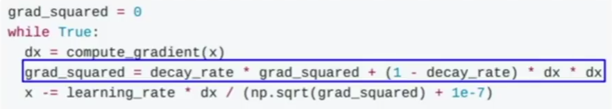
The term decay_rate is used to apply exponential smoothing on grad_squared term.
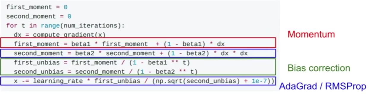
Adam optimization
Adam is a combination of Momentum and RMSprop.
Normal equation
To minimize the cost function \(J(╬Ė) = \frac{1}{2} \sum_{i=1}^{n} (y^{(i)}-h_{╬Ė}(x^{(i)}))^{2} = \frac{1}{2} (X╬Ė – y)^T(X╬Ė – y)\), we need to solve the equation:
\( \frac{\partial J(╬Ė)}{\partial ╬Ė} = 0 \\ \frac{\partial trace(J(╬Ė))}{\partial ╬Ė} = 0 \\ \frac{\partial trace((X╬Ė – y)^T(X╬Ė – y))}{\partial ╬Ė} = 0 \\ \frac{\partial trace(╬Ė^TX^TX╬Ė – ╬Ė^TX^Ty – y^TX╬Ė + y^Ty)}{\partial ╬Ė} = 0\) \(\frac{\partial trace(╬Ė^TX^TX╬Ė) – trace(╬Ė^TX^Ty) – trace(y^TX╬Ė) + trace(y^Ty))}{\partial ╬Ė} = 0 \\ \frac{\partial trace(╬Ė^TX^TX╬Ė) – trace(╬Ė^TX^Ty) – trace(y^TX╬Ė))}{\partial ╬Ė} = 0\) \(\frac{\partial trace(╬Ė^TX^TX╬Ė) – trace(y^TX╬Ė) – trace(y^TX╬Ė))}{\partial ╬Ė} = 0 \\ \frac{\partial trace(╬Ė^TX^TX╬Ė) – 2 trace(y^TX╬Ė))}{\partial ╬Ė} = 0 \\ \frac{\partial trace(╬Ė╬Ė^TX^TX)}{\partial ╬Ė} – 2 \frac{\partial trace(╬Ėy^TX))}{\partial ╬Ė} = 0 \\ 2 X^TX╬Ė – 2 X^Ty = 0 \\ X^TX╬Ė= X^Ty \\ ╬Ė = {(X^TX)}^{-1}X^Ty\)If \(X^TX\) is singular, then we need to calculate the pseudo inverse instead of the inverse.
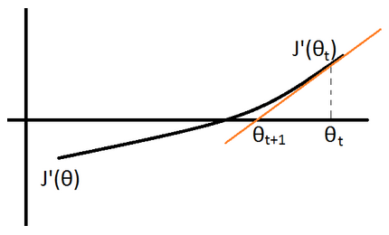
Newton method
Matrix differentiation
To minimize the cost function: \(J(╬Ė) = \frac{1}{2} \sum_{i=1}^{n} (y^{(i)}-h_{╬Ė}(x^{(i)}))^{2} = \frac{1}{2} (X╬Ė – y)^T(X╬Ė – y)\), we need to solve the equation:
\( \frac{\partial J(╬Ė)}{\partial ╬Ė} = 0 \\ \frac{\partial ╬Ė^TX^TX╬Ė – ╬Ė^TX^Ty – y^TX╬Ė + y^Ty}{\partial ╬Ė} = 2X^TX╬Ė – \frac{\partial ╬Ė^TX^Ty}{\partial ╬Ė} – X^Ty = 0\)\(2X^TX╬Ė – \frac{\partial y^TX╬Ė}{\partial ╬Ė} – X^Ty = 2X^TX╬Ė – 2X^Ty = 0\) (Note: In matrix differentiation: \( \frac{\partial A╬Ė}{\partial ╬Ė} = A^T\) and \( \frac{\partial ╬Ė^TA╬Ė}{\partial ╬Ė} = 2A^T╬Ė\))
we can deduce \(X^TX╬Ė = X^Ty\) and \(╬Ė = (X^TX)^{-1}X^Ty\)
Logistic Regression
Below a table that shows tumor types by size.
|
x = Tumor Size (cm) |
y = Tumor Type (Benign=0, Malignant=1) |
|
1 |
0 |
|
1 |
0 |
|
2 |
0 |
|
2 |
1 |
|
3 |
1 |
|
3 |
1 |
Given x, y is distributed according to the Bernoulli distribution with probability of success p = E[y|x].
\(P(y|x;╬Ė) = p^y (1-p)^{(1-y)}\)We define h(x) as a function that returns the expected value (p) of the distribution. We will define this function as:
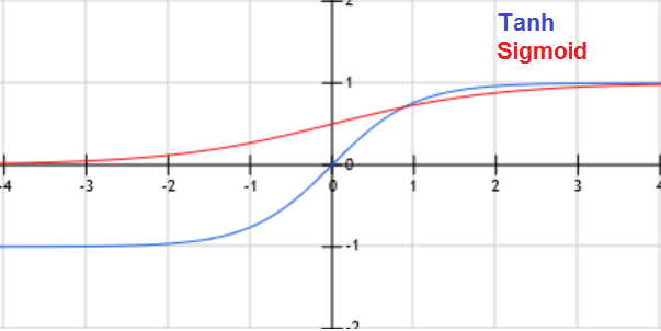
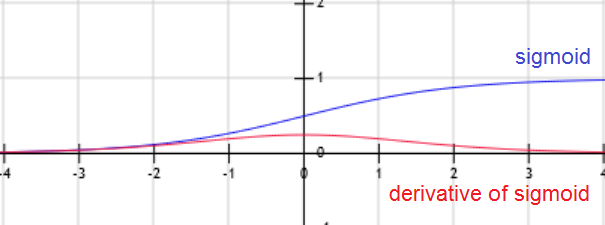
\(E[y|x] = h_{╬Ė}(x) = g(╬Ė^T x) = \frac{1}{1+exp(-╬Ė^T x)}\). g is called Sigmoid (or logistic) function.
P(y|x; ╬Ė) = \(h_{╬Ė}(x)^y (1-h_{╬Ė}(x))^{(1-y)}\)
We need to find ╬Ė that maximizes this probability for all values of x. In other words, we need to find ╬Ė that maximizes the likelihood function L:
\(L(╬Ė)=P(\overrightarrow{y}|X;╬Ė)=\prod_{i=1}^{m} P(y^{(i)}|x^{(i)};╬Ė)\)Or maximize the log likelihood function l:
\(l(╬Ė)=log(L(╬Ė)) = \sum_{i=1}^{m} log(P(y^{(i)}|x^{(i)};╬Ė ))\) \(= \sum_{i=1}^{m} y^{(i)} log(h_{╬Ė}(x^{(i)}))+ (1-y^{(i)}) log(1-h_{╬Ė}(x^{(i)}))\)Or minimize the \(-l(╬Ė) = \sum_{i=1}^{m} -y^{(i)} log(h_{╬Ė}(x^{(i)})) – (1-y^{(i)}) log(1-h_{╬Ė}(x^{(i)})) = J(╬Ė) \)
J(╬Ė) is convex, to minimize it, we need to solve the equation \(\frac{\partial J(╬Ė)}{\partial ╬Ė} = 0\).
There are many methods to solve this equation:
- Gradient descent
Gradient descent
\(╬Ė_{j} := ╬Ė_{j} – ╬▒ \sum_{i=1}^{n} (h_{╬Ė}(x^{(i)}) – y^{(i)}) * x_j^{(i)} \)Logit function (inverse of logistic function)
Logit function is defined as follow: \(logit(p) = log(\frac{p}{1-p})\)
The idea in the use of this function is to transform the interval of p (outcome) from [0,1] to [0, Ōł×]. So instead of applying linear regression on p, we will apply it on logit(p).
Once we find ╬Ė that maximizes the Likelihood function, we can then estimate logit(p) given a value of x (\(logit(p) = h_{╬Ė}(x) \)). p can be then calculated using the following formula:
\(p = \frac{1}{1+exp(-logit(h_{╬Ė}(x)))}\)Multinomial Logistic Regression (using maximum likelihood estimation)
In multinomial logistic regression (also called Softmax Regression), y could have more than two outcomes {1,2,3,…,k}.
Below a table that shows tumor types by size.
|
x = Tumor Size (cm) |
y = Tumor Type (Type1= 1, Type2= 2, Type3= 3) |
|
1 |
1 |
|
1 |
1 |
|
2 |
2 |
|
2 |
2 |
|
2 |
3 |
|
3 |
3 |
|
3 |
3 |
Given x, we can define a multinomial distribution with probabilities of success \(\phi_j = E[y=j|x]\).
\(P(y=j|x;\Theta) = ŽĢ_j \\ P(y=k|x;\Theta) = 1 – \sum_{j=1}^{k-1} ŽĢ_j \\ P(y|x;\Theta) = ŽĢ_1^{1\{y=1\}} * … * ŽĢ_{k-1}^{1\{y=k-1\}} * (1 – \sum_{j=1}^{k-1} ŽĢ_j)^{1\{y=k\}}\)We define \(\tau(y)\) as a function that returns a \(R^{k-1}\) vector with value 1 at the index y: \(\tau(y) = \begin{bmatrix}0\\0\\1\\0\\0\end{bmatrix}\), when \(y \in \{1,2,…,k-1\}\), .
and \(\tau(y) = \begin{bmatrix}0\\0\\0\\0\\0\end{bmatrix}\), when y = k.
We define \(\eta(x)\) as a \(R^{k-1}\) vector = \(\begin{bmatrix}log(\phi_1/\phi_k)\\log(\phi_2/\phi_k)\\…\\log(\phi_{k-1}/\phi_k)\end{bmatrix}\)
\(P(y|x;\Theta) = 1 * exp(╬Ę(x)^T * \tau(y) – (-log(\phi_k)))\)This form is an exponential family distribution form.
We can invert \(\eta(x)\) and find that:
\(ŽĢ_j = ŽĢ_k * exp(╬Ę(x)_j)\) \(= \frac{1}{1 + \frac{1-ŽĢ_k}{ŽĢ_k}} * exp(╬Ę(x)_j)\) \(=\frac{exp(╬Ę(x)_j)}{1 + \sum_{c=1}^{k-1} ŽĢ_c/ŽĢ_k}\) \(=\frac{exp(╬Ę(x)_j)}{1 + \sum_{c=1}^{k-1} exp(╬Ę(x)_c)}\)If we define ╬Ę(x) as linear function, \(╬Ę(x) = ╬ś^T x = \begin{bmatrix}╬ś_{1,1} x_1 +… + ╬ś_{n,1} x_n \\╬ś_{1,2} x_1 +… + ╬ś_{n,2} x_n\\…\\╬ś_{1,k-1} x_1 +… + ╬ś_{n,k-1} x_n\end{bmatrix}\), and ╬ś is a \(R^{n*(k-1)}\) matrix.
Then: \(ŽĢ_j = \frac{exp(╬ś_j^T x)}{1 + \sum_{c=1}^{k-1} exp(╬ś_c^T x)}\)
The hypothesis function could be defined as: \(h_╬ś(x) = \begin{bmatrix}\frac{exp(╬ś_1^T x)}{1 + \sum_{c=1}^{k-1} exp(╬ś_c^T x)} \\…\\ \frac{exp(╬ś_{k-1}^T x)}{1 + \sum_{c=1}^{k-1} exp(╬ś_c^T x)} \end{bmatrix}\)
We need to find ╬ś that maximizes the probabilities P(y=j|x;╬ś) for all values of x. In other words, we need to find ╬Ė that maximizes the likelihood function L:
\(L(╬Ė)=P(\overrightarrow{y}|X;╬Ė)=\prod_{i=1}^{m} P(y^{(i)}|x^{(i)};╬Ė)\) \(=\prod_{i=1}^{m} \phi_1^{1\{y^{(i)}=1\}} * … * \phi_{k-1}^{1\{y^{(i)}=k-1\}} * (1 – \sum_{j=1}^{k-1} \phi_j)^{1\{y^{(i)}=k\}}\) \(=\prod_{i=1}^{m} \prod_{c=1}^{k-1} \phi_c^{1\{y^{(i)}=c\}} * (1 – \sum_{j=1}^{k-1} \phi_j)^{1\{y^{(i)}=k\}}\)\(=\prod_{i=1}^{m} \prod_{c=1}^{k-1} \phi_c^{1\{y^{(i)}=c\}} * (1 – \sum_{j=1}^{k-1} \phi_j)^{1\{y^{(i)}=k\}}\) and \(ŽĢ_j = \frac{exp(╬ś_j^T x)}{1 + \sum_{c=1}^{k-1} exp(╬ś_c^T x)}\)
Multinomial Logistic Regression (using cross-entropy minimization)
In this section, we will try to minimize the cross-entropy between Y and estimated \(\widehat{Y}\).
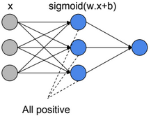
We define \(W \in R^{d*n}\), \(b \in R^{d}\) such as \(S(W x + b) = \widehat{Y}\), S is the Softmax function, k is the number of outputs, and \(x \in R^n\).
To estimate W and b, we will need to minimize the cross-entropy between the two probability vectors Y and \(\widehat{Y}\).
The cross-entropy is defined as below:
\(D(\widehat{Y}, Y) = -\sum_{j=1}^d Y_j Log(\widehat{Y_j})\)Example:
if \(\widehat{y} = \begin{bmatrix}0.7 \\0.1 \\0.2 \end{bmatrix} \& \ y=\begin{bmatrix}1 \\0 \\0 \end{bmatrix}\) then \(D(\widehat{Y}, Y) = D(S(W x + b), Y) = -1*log(0.7)\)
We need to minimize the entropy for all training examples, therefore we will need to minimize the average cross-entropy of the entire training set.
\(L(W,b) = \frac{1}{m} \sum_{i=1}^m D(S(W x^{(i)} + b), y^{(i)})\), L is called the loss function.
If we define \(W = \begin{bmatrix} — ╬Ė_1 — \\ — ╬Ė_2 — \\ .. \\ — ╬Ė_d –\end{bmatrix}\) such as:
\(╬Ė_1=\begin{bmatrix}╬Ė_{1,0}\\╬Ė_{1,1}\\…\\╬Ė_{1,n}\end{bmatrix}, ╬Ė_2=\begin{bmatrix}╬Ė_{2,0}\\╬Ė_{2,1}\\…\\╬Ė_{2,n}\end{bmatrix}, ╬Ė_d=\begin{bmatrix}╬Ė_{d,0}\\╬Ė_{d,1}\\…\\╬Ė_{d,n}\end{bmatrix}\)We can then write \(L(W,b) = \frac{1}{m} \sum_{i=1}^m D(S(W x^{(i)} + b), y^{(i)})\)
\(= \frac{1}{m} \sum_{i=1}^m \sum_{j=1}^d 1^{\{y^{(i)}=j\}} log(\frac{exp(╬Ė_k^T x^{(i)})}{\sum_{k=1}^d exp(╬Ė_k^T x^{(i)})})\)For d=2 (nbr of class=2), \(= \frac{1}{m} \sum_{i=1}^m 1^{\{y^{(i)}=\begin{bmatrix}1 \\ 0\end{bmatrix}\}} log(\frac{exp(╬Ė_1^T x^{(i)})}{exp(╬Ė_1^T x^{(i)}) + exp(╬Ė_2^T x^{(j)})}) + 1^{\{y^{(i)}=\begin{bmatrix}0 \\ 1\end{bmatrix}\}} log(\frac{exp(╬Ė_2^T x^{(i)})}{exp(╬Ė_1^T x^{(i)}) + exp(╬Ė_2^T x^{(i)})})\)
\(1^{\{y^{(i)}=\begin{bmatrix}1 \\ 0\end{bmatrix}\}}\) means that the value is 1 if \(y^{(i)}=\begin{bmatrix}1 \\ 0\end{bmatrix}\) otherwise the value is 0.
To estimate \(╬Ė_1,…,╬Ė_d\), we need to calculate the derivative and update \(╬Ė_j = ╬Ė_j – ╬▒ \frac{\partial L}{\partial ╬Ė_j}\)
Kernel regression
Kernel regression is a non-linear model. In this model we define the hypothesis as the sum of kernels.
\(\widehat{y}(x) = ŽĢ(x) * ╬Ė = ╬Ė_0 + \sum_{i=1}^d K(x, ╬╝_i, ╬╗) ╬Ė_i \) such as:
\(ŽĢ(x) = [1, K(x, ╬╝_1, ╬╗),…, K(x, ╬╝_d, ╬╗)]\) and \(╬Ė = [╬Ė_0, ╬Ė_1,…, ╬Ė_d]\)
For example, we can define the kernel function as : \(K(x, ╬╝_i, ╬╗) = exp(-\frac{1}{╬╗} ||x-╬╝_i||^2)\)
Usually we select d = number of training examples, and \(╬╝_i = x_i\)
Once the vector ŽĢ(X) calculated, we can use it as new engineered vector, and then use the normal equation to find ╬Ė:
\(╬Ė = {(ŽĢ(X)^TŽĢ(X))}^{-1}ŽĢ(X)^Ty\)Bayes Point Machine
The Bayes Point Machine is a Bayesian linear classifier that can be converted to a nonlinear classifier by using feature expansions or kernel methods as the Support Vector Machine (SVM).
More details will be provided.
Ordinal Regression
Ordinal Regression is used for predicting an ordinal variable. An ordinal variable is a categorical variable for which the possible values are ordered (eg. size: Small, Medium, Large).
More details will be provided.
Poisson Regression
Poisson regression assumes the output variable Y has a Poisson distribution, and assumes the logarithm of its expected value can be modeled by a linear function.
log(E[Y|X]) = log(╬╗) = ╬Ė.x