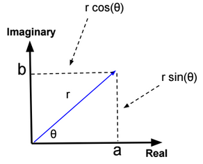
Basic Statistics
Basic statistics for a discrete variable X:
|
Mean(μ) = Expect Value E[X] |
=\(\frac{1}{n} \sum_{i=1}^{n} x_{i} \) |
|
Median |
If n is odd then \(x_{\frac{n+1}{2}}\) else \(\frac{x_{\frac{n}{2}} + x_{\frac{n+2}{2}}}{2}\) |
|
Variance (\(\sigma^{2}=E_{x \sim p(x)}[(X-E[X])^2]\)) (n-1 is called degree of freedom) |
=\(\frac{1}{n-1}\sum_{i=1}^{n} (x_{i} -\mu)^{2}\) |
|
Standard deviation (\(\sigma\)) |
=\(\sqrt{\sigma^{2}}\) |
|
Mode |
is the value x at which its probability mass function takes its maximum value. For example the mode of {1,1,1,2,2,3,4} is 1 because it appears 3 times |
|
Covariance(X,Y) |
\(= E[(X-E[X])(Y-E[Y])]\) \(= E[XY] -E[X]E[Y]\) \(= \frac{1}{n-1} \sum_{i=1}^{n} (X_i – μ_X)(Y_i – μ_Y)\) |
|
Correlation(X,Y) |
=\(\frac{Covariance(X,Y)}{\sqrt{Var(X).Var(Y)}}\) |
|
Standard error |
\(= \frac{σ}{\sqrt{n}}\) |
Basic statistics for a continuous variable X:
|
Mean(μ) = Expect Value E[X] |
=\(\int_{all\, x} p(x)\,x\,dx\) |
|
Median |
m such as p(x<=m) = .5 |
|
Variance (\(\sigma^{2}=E_{x \sim p(x)}[(X-E[X])^2]\)) |
=\(\int_{all\, x} p(x)\,(x -\mu)^{2}\,dx\) |
|
Standard deviation (\(\sigma\)) |
=\(\sqrt{\sigma^{2}}\) |
|
Mode |
is the value x at which its probability density function has its maximum value |
Examples:
For a set {-1, -1, 1, 1} => Mean = 0, Variance = 1.33, Standard deviation = 1.15
If \(x \in [0, +\infty]\) and p(x) = exp(-x) => Mean = 1, Variance = 1, Standard deviation = 1
Expected value
Expectations are linear. E[X+Y] = E[X] + E[Y]
Probability Distributions
A random variable is a set of outcomes from a random experiment.
A probability distribution is a function that returns the probability of occurrence of an outcome. For discrete random variables, this function is called “Probability Mass Function”. For continuous variables, this function is called “Probability Density Function”.
A joint probability distribution is a function that returns the probability of joint occurrence of outcomes from two or more random variables. If random variables are independent then the joint probability distribution is equal to the product of the probability distribution of each random variable.
A conditional probability distribution is the probability distribution of a random variable given another random variables.
Example:
|
X |
P(X) |
|
A |
0.2 |
|
B |
0.8 |
P(X) is the probability distribution of X.
|
Y |
P(Y) |
|
C |
0.1 |
|
D |
0.9 |
P(Y) is the probability distribution of Y.
|
X |
Y |
P(X,Y) |
|
A |
C |
0.1 |
|
A |
D |
0.1 |
|
B |
D |
0.8 |
P(X,Y) is the joint probability distribution of X and Y.
|
X |
P(X|Y=D) = P(X,Y)/P(Y=D) |
|
A |
0.1/0.9 |
|
B |
0.8/0.9 |
P(X|Y=D) is the conditional probability distribution of X given Y = D.
Marginal probability
Sometimes we know the probability distribution over a set of variables and we want to know the probability distribution over just a subset of them. The probability distribution over the subset is known as the marginal probability distribution.
For example, suppose we have discrete random variables x and y, and we know P(x, y). We can find P(x) with the sum rule: \(P(x) = \sum_y P(x,y)\)
Below the statistical properties of some distributions.
Binomial distribution
Nb of output values = 2 (like coins)
n = number of trials
p = probability of success
P(X) = \(C_n^X * p^{X} * (1-p)^{n-X}\)
Expected value = n.p
Variance = n.p.(1-p)
Example:
If we flip a fair coin (p=0.5) three time (n=3), what’s the probability of getting two heads and one tail?
P(X=2) = P(2H and 1T) = P(HHT + HTH + THH) = P(HHT) + P(HTH) + P(THH) = p.p(1-p) + p.(1-p).p + (1-p).p.p = \(C_3^2.p^2.(1-p)\)
Bernoulli distribution
Bernoulli distribution is a special case of the binomial distribution with n=1.
Nb of output values = 2 (like coins)
n = 1 (number of trials)
p = probability of success
X \(\in\) {0,1}
P(X) = \(p^{X} * (1-p)^{1-X}\)
Expected value = p
Variance = p.(1-p)
Example:
If we flip a fair coin (p=0.5) one time (n=1), what’s the probability of getting 0 head?
P(X=0) = P(0H) = P(1T) = 1-p = \(p^0.(1-p)^1\)
Multinomial distribution
It’s a generalization of Binomial distribution. In a Multinomial distribution we can have more than two outcomes. For each outcome, we can assign a probability of success.
Normal (Gaussian) distribution
P(x) = \(\frac{1}{\sigma \sqrt{2\pi}} exp(-\frac{1}{2} (\frac{x-\mu}{\sigma})^{2})\)
σ and μ are sufficient statistics (sufficient to describe the whole curve)
Expected value = \(\int_{-\infty}^{+\infty} p(x) x \, dx\)
Variance = \(\int_{-\infty}^{+\infty} (x – \mu)^2 p(x) \, dx\)
Standard Normal distribution (Z-Distribution)
It’s a normal distribution with mean = 0 and standard deviation = 1.
P(z) = \(\frac{1}{\sqrt{2\pi}} exp(-\frac{1}{2} z^2)\)
Cumulative distribution function:
\(P(x \leq z) = \int_{-\infty}^{z} \frac{1}{\sqrt{2\pi}} exp(-\frac{1}{2} x^2) \, dx\)Exponential Family distribution
\(P(x;\theta) = h(x)\exp \left(\eta (θ)\cdot T(x)-A(θ)\right) \), where T(x), h(x), η(θ), and A(θ) are known functions.
θ = vector of parameters.
T(x) = vector of “sufficient statistics”.
A(θ) = cumulant generating function.
The Binomial distribution is an Exponential Family distribution
\(P(x)=C_n^x\ p^{x}(1-p)^{n-x},\quad x\in \{0,1,2,\ldots ,n\}\)This can equivalently be written as:
\(P(x)=C_n^x\ exp (log(\frac{p}{1-p}).x – (-n.log(1-p)))\)The Normal distribution is an Exponential Family distribution
Consider a random variable distributed normally with mean μ and variance \(σ^2\). The probability density function could be written as: \(P(x;θ) = h(x)\exp(η(θ).T(x)-A(θ)) \)
With:
\(h(x)={\frac{1}{\sqrt {2\pi \sigma ^{2}}}}exp^{-{\frac {x^{2}}{2\sigma ^{2}}}}\) \(T(x)={\frac {x}{\sigma }}\) \(A(\mu)={\frac {\mu ^{2}}{2\sigma ^{2}}}\) \(\eta(\mu)={\frac {\mu }{\sigma }}\)Poisson distribution
The Poisson distribution is popular for modelling the number of times an event occurs in an interval of time or space (eg. number of arrests, number of fish in a trap…).
In a Poisson distribution, values are discrete and can’t be negative.
The probability mass function is defined as: \(P(x=k)=\frac{λ^k.e^{-λ}}{k!}\), k is the number of occurrences. λ is the expected number of occurrences.
Exponential distribution
The exponential distribution has a probability distribution with a sharp point at x = 0.
\(P(x; λ) = λ.1_{x≥0}.exp (−λx)\)Laplace distribution
Laplace distribution has a sharp peak of probability mass at an arbitrary point μ. The probability mass function is defined as \(Laplace(x;μ,γ) = \frac{1}{2γ} exp(-\frac{|x-μ|}{γ})\)
Laplace distribution is a distribution that is symmetrical and more “peaky” than a normal distribution. The dispersion of the data around the mean is higher than that of a normal distribution. Laplace distribution is also sometimes called the double exponential distribution.
Dirac distribution
The probability mass function is defined as \(P(x;μ) = δ(x).(x-μ)\) such as δ(x) = 0 when x ≠ μ and \(\int_{-∞}^{∞} δ(x).(x-μ) dx= 1\).
Empirical Distribution
Other known Exponential Family distributions
Dirichlet.
Laplace Smoothing
Given a set S={a1, a1, a1, a2}.
Laplace smoothed estimate for P(x) with domain of x in {a1, a2, a3}:
\(P(x=a1)=\frac{3 + 1}{4 + 3}\) \(P(x=a2)=\frac{1 + 1}{4 + 3}\) \(P(x=a3)=\frac{0 + 1}{4 + 3}\)Maximum Likelihood Estimation
Given three independent data points \(x_1=1, x_2=0.5, x_3=1,5\), what the mean μ of a normal distribution that these three points are more likely to come from (we suppose the variance=1).
If μ = 4, then the probabilities \(P(X=x_1), P(X=x_2), P(X=x_3)\) will be low, and \(P(x_1,x_2,x_3) = P(X=x_1)*P(X=x_2)*P(X=x_3)\) will be also low.
If μ = 1, then the probabilities \(P(X=x_1), P(X=x_2), P(X=x_3)\) will be high, and \(P(x_1,x_2,x_3) = P(X=x_1)*P(X=x_2)*P(X=x_3)\) will be also high. Which means that the three points are more likely to come from a normal distribution with mean μ = 1.
The likelihood function is defined as: \(P(x_1,x_2,x_3; μ)\)
Central Limit Theorem
The central limit theorem states that if you have a population with mean μ and standard deviation σ and take sufficiently large random samples from the population with replacement , then the distribution of sample means will be approximately normally distributed.
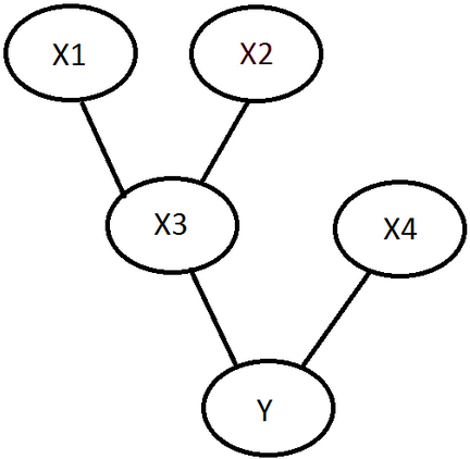
Bayesian Network
X1, X2 are random variables.
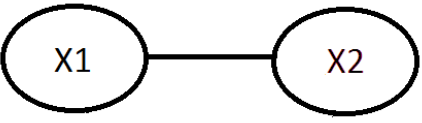
P(X1,X2) = P(X2,X1) = P(X2|X1) * P(X1) = P(X1|X2) * P(X2)
P(X1) is called prior probability.
P(X1|X2) is called posterior probability.
Example:
A mixed school having 60% boys and 40% girls as students. The girls wear trousers or skirts in equal numbers; the boys all wear trousers. An observer sees from a distance a student wearing a trouser. What is the probability this student is a girl?
The prior probability P(Girl): 0.4
The posterior probability P(Girl|Trouser): \(\frac{P(Trouser|Girl)*P(Girl)}{P(Trouser|Girl) * P(Girl) + P(Trouser|Boy) * P(Boy)} = 0.25\)
Parameters estimation – Bayesian Approach Vs Frequentist Approach
There are two approaches that can be used to estimate the parameters of a model.
|
Frequentist approach |
Bayesian approach |
| \(arg\ \underset{θ}{max} \prod_{i=1}^m P(y^{(i)}|x^{(i)};θ)\) |
\(arg\ \underset{θ}{max} P(θ|\{(x^{(i)}, y^{(i)})\}_{i=1}^m)\)
\(=arg\ \underset{θ}{max} \frac{P(\{(x^{(i)}, y^{(i)})\}_{i=1}^m|θ) * P(θ)}{P(\{(x^{(i)}, y^{(i)})\}_{i=1}^m)}\)
\(=arg\ \underset{θ}{max} P(\{(x^{(i)}, y^{(i)})\}_{i=1}^m|θ) * P(θ)\)
If \(\{(x^{(i)}, y^{(i)})\}\) are independent, then: \(=arg\ \underset{θ}{max} \prod_{i=1}^m P((y^{(i)},x^{(i)})|θ) * P(θ)\)To calculate P(θ) (called the prior), we assume that θ is Gaussian with mean 0 and variance \(\sigma^2\). \(=arg\ \underset{θ}{max} log(\prod_{i=1}^m P((y^{(i)},x^{(i)})|θ) * P(θ))\) \(=arg\ \underset{θ}{max} log(\prod_{i=1}^m P((y^{(i)},x^{(i)})|θ)) + log(P(θ))\)after some few derivations, we will find the the expression is equivalent to the L2 regularized linear cost function. \(=arg\ \underset{θ}{min} \frac{1}{2} \sum_{i=1}^{n} (y^{(i)}-h_{θ}(x^{(i)}))^{2} + λ θ^Tθ\) |
Because of the prior, Bayesian algorithms are less susceptible to overfitting.
Cumulative distribution function (CDF)
Given a random continuous variable S with density function p(s). The Cumulative distribution function \(F(s) = p(S<=s) = \int_{-∞}^{s} p(s) ds\)
F'(s) = p(s)