This post describes some geometric machine learning algorithms.
K-Nearest Neighbor Regression
k-nearest neighbors regression algorithm (k-NN regression) is a non-parametric method used for regression. For a new example x, predict y as the average of values \(y_1, y_2, …, y_k\) of k nearest neighbors of x.
K-Nearest Neighbor Classifier
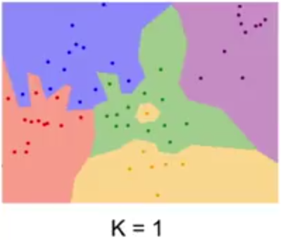
k-nearest neighbors classifier (k-NN classifier) is a non-parametric method used for classification. For a new example x, predict y as the most common class among the k nearest neighbors of x.
Support Vector Machine (SVM)
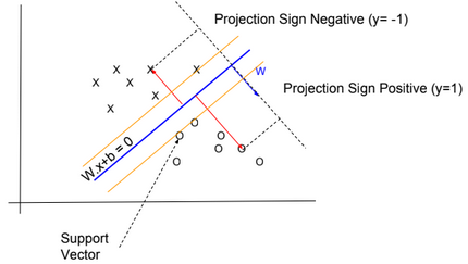
In SVM, y has two values -1 or 1, and the hypothesis function is \(h_{W,b}(x) = g(W^T x + b)\) with g(z) = {1 if z >= 0, otherwise -1}.
We need to find W and b so \(W^T x + b\) >> 0 when y=1 and \(W^T x + b\) << 0 when y=-1
Functional margin
\(\widehat{?}^{(i)} = y^{(i)} . (W^T x^{(i)} +b)\)We want that this function be >> 0 for all values of x.
We define \(\widehat{?} = min \ \widehat{?}^{(i)}\) for all values of i
Geometric margin
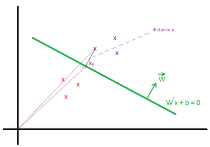
Geometric margin \(?^{(i)}\) is the geometric distance between an example \(x^{(i)}\) and the line defined by \(W^Tx + b = 0\). We define \(x_p^{(i)}\) as the point of projection of \(x^{(i)}\) on the line.
The vector \(\overrightarrow{x}^{(i)} = \overrightarrow{x_p}^{(i)} + ?^{(i)} * \frac{\overrightarrow{W}}{||W||} \)
\(x_p^{(i)}\) is in the line, then \(W^T (x^{(i)} – ?^{(i)} * \frac{W}{||W||}) + b = 0\)
We can find that \(?^{(i)} = \frac{W^T x^{(i)} + b}{||W||} \)
More generally \(?^{(i)} = y^{(i)}(\frac{W^T x^{(i)}}{||W||} + \frac{b}{||W||}) \)
We define \(? = min {?}^{(i)}\) for all values of i
We can deduce that the Geometric margin(?) = Functional margin / ||W||
Max Margin Classifier
We need to maximize the geometric margin \(?\), in other words \(\underset{W, b, ?}{max}\) ?, such as \(y^{(i)}(\frac{W^T x^{(i)}}{||W||} + \frac{b}{||W||})\) >= ? for all values \((x^{(i)},y^{(i)})\).
To simplify the maximization problem, we impose a scaling constraint: \(\widehat{?} = ? * ||W|| = 1\).
The optimization problem becomes as follow: \(\underset{W, b}{max}\frac{1}{||W||}\) (or \(\underset{W, b}{min}\frac{1}{2}||W||^2\)), such as \(y^{(i)}(W^T x^{(i)} + b)\) >= 1 for all values \((x^{(i)},y^{(j)})\).
Using the method of Lagrange Multipliers, we can solve the minimization problem.
\(L(W, b, ?) = \frac{1}{2} ||W||^2 – \sum_{i=1}^m ?_i * (y^{(i)}(W^T x^{(i)} + b) – 1)\)Based on the KKT conditions, \(?_i >= 0\) and \(?_i * (y^{(i)}(W^T x^{(i)} + b) – 1) = 0\) for all i.
We know that \(y^{(i)}(W^T x^{(i)} + b) – 1 = 0\) is true only for few examples (called support vectors) located close to the the line \(W^Tx + b = 0\) (for these examples, \(? = {?}^{(i)} = \frac{1}{||W||}\)), therefore \(?_i\) is equal to 0 for the majority of examples.
By deriving L, we can find:
\(\frac{\partial L(W, b, ?)}{\partial w} = W – \sum_{i=1}^m ?_i * y^{(i)} * x^{(i)} = 0 \\ \frac{\partial L(W, b, ?)}{\partial b} = \sum_{i=1}^m ?_i * y^{(i)} = 0\)After multiple derivations, we can find the equations for W, b and ?.
More details can be found in this video: https://www.youtube.com/watch?v=s8B4A5ubw6c
Predictions
The hypothesis function is defined as: \(h_{W,b}(x) = g(W^T x + b) = g(\sum_{i=1}^m ?_i * y^{(i)} * K(x^{(i)}, x) + b) \)
The function \(K(x^{(i)}, x) = ?(x^{(i)})^T ?(x) \) is known as the kernel function (? is a mapping function).
When ?(x) = x, then \(h_{W,b}(x) = g(\sum_{i=1}^m ?_i * y^{(i)} * (x^{(i)})^T . x + b) \)
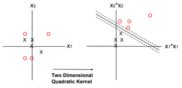
Kernels
There are many types of kernels: �Polynomial kernel�, �Gaussian kernel�,…
In the example below the kernel is defined as Quadratic Kernel. \(K(x^{(i)}, x) = ?(x^{(i)})^T ?(x)\) and \(?(x) = (x_1^2, x_2^2, \sqrt{2} x_1 x_2)\). By using this kernel, SVM can find a linear separator (or hyperplane).
Regularization
Regularization can be applied to SVM by adding an extra term to the minimization function. The extra term relaxes the constraints by introducing slack variables. C is the regularization parameter.
\(\underset{W, b, ?_i}{min}\frac{||W||^2}{2} \color{red} {+ C \sum_{i=1}^m ?_i }\), such as \(y^{(i)}(W^T x^{(i)} + b)\) >= 1 – ?i for all values \((x^{(i)},y^{(j)})\) and \(?_i >= 0\).
The regularization parameter serves as a degree of importance that is given to miss-classifications. SVM poses a quadratic optimization problem that looks for maximizing the margin between both classes and minimizing the amount of miss-classifications. However, for non-separable problems, in order to find a solution, the miss-classification constraint must be relaxed.
As C grows larger, wrongly classified examples are not allowed, and when C tends to zero the more miss-classifications are allowed.
One-Class SVM
One-Class SVM is used to detect outliers. It finds a minimal hypersphere around the data. In other words, we need to minimize the radius R.
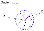
The minimization function for this model is defined as follow:
\(\underset{R, a, ?_i}{min} ||R||^2 + C \sum_{i=1}^m ?_i \), such as \(||x^{(i)} – a||^2 \leq R^2 + ?i\) for all values \((x^{(i)},y^{(j)})\) and \(?_i >= 0\).
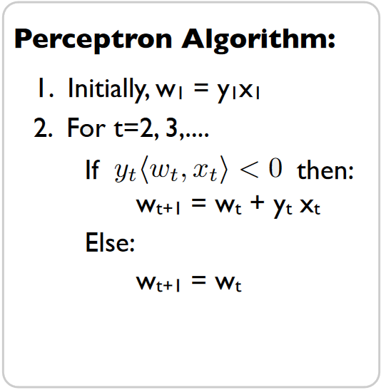
Perceptron Algorithm
Similar to SVM, the Perceptron algorithm tries to separate positive and negative examples. There is no notion of kernel or margin maximization when using the perceptron algorithm. The algorithm can be trained online.
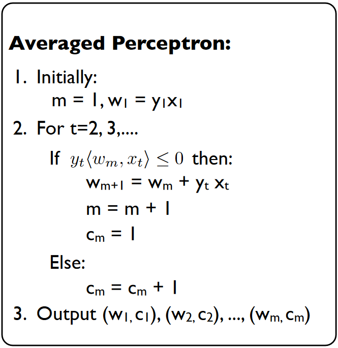
Averaged Perceptron Algorithm
Averaged Perceptron Algorithm is an extension of the standard Perceptron algorithm; it uses averaged weights and biases.
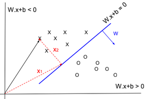
The classification of a new example is calculated by evaluating the following expression:
\(? = sign(\sum_{i=1}^m c_i.w_i^T.x + b_i)\)Note: the sign of wx+b is related to the location of the point x.
w.x+b = w(x1+x2)+b = w.x2 because x1 is located on the blue line then w.x1+b = 0.
w.x2 is positive if the two vectors have the same direction.
K-means
Given a training set \(S = \{x^{(i)}\}_{i=1}^m\). We define k as the number of clusters (groups) to create. Each cluster has a centroid \(\mu_k\).
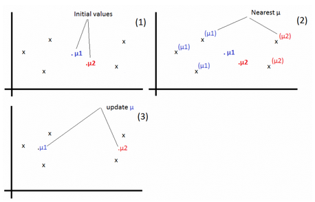
1-For each example, find j that minimizes: \(c^{(i)} := arg\ \underset{j}{min} ||x^{(i)} – \mu_j||^2\)
2-Update \(\mu_j:=\frac{\sum_{i=1}^m 1\{c^{(i)} = j\} x^{(i)}}{\sum_{i=1}^m 1\{c^{(i)} = j\}}\)
Repeat the operations 1 & 2 until convergence.