Linear Algebra

A matrix is a 2-D array of numbers.

A tensor is a n-D array of numbers.

Matrices are associative but not commutative.

Not all square matrices have inverse. A matrix that is not invertible is called Singular or Degenerative.

A matrix is “singular” if any of the following are true:

-Any row or column contains all zeros.

-Any two rows or columns are identical.

-Any row or column is a linear combination of other rows or columns.

A square matrix A is singular, if and only if the determinant(A) = 0

Inner product of two vectors \(\overrightarrow{u}\) and \(\overrightarrow{v}\):

\(\overrightarrow{u} * \overrightarrow{v} = p * ||\overrightarrow{u}|| = p * \sqrt{\sum_{i=1}^{n}u_{i}^{2}} = u^{T} * v = \sum_{i=1}^{n}u_{i} * v_{i}\)

p is the projection of \(\overrightarrow{v}\) on \(\overrightarrow{u}\) and \(||\overrightarrow{u}||\) is the Euclidean norm of \(\overrightarrow{u}\).

\(A = \begin{bmatrix} a & b & c\\ d & e & f\\ g & h & i \end{bmatrix}\)

Determinant(A) = |A| = a(ei-hf) – b(di-gf) + c(dh – ge)

If \(f: R^{n*m} \mapsto R\)

\(\frac{\partial}{\partial A} f(A) = \begin{bmatrix} \frac{\partial}{\partial a_{11}}f(A) & … & \frac{\partial}{\partial a_{1m}} f(A)\\ … & … & …\\ \frac{\partial}{\partial a_{n1}}f(A) & … & \frac{\partial}{\partial a_{nm}}A\\ \end{bmatrix}\)

Example:

\( f(A) = a_{11} + … + a_{nm} \)

\(\frac{\partial}{\partial A} f(A) = \begin{bmatrix} 1 & … & 1\\ … & … & …\\ 1 & … & 1 \\ \end{bmatrix}\)

If A is a squared matrix:

trace(A) = \(\sum_{i=1}^n A_{ii}\)

trace(AB) = trace(BA)

trace(ABC) = trace(CAB) = trace(BCA)

trace(B) = trace(\(B^T\))

trace(a) = a

\(\frac{\partial}{\partial A} trace(AB) = B^T\) \(\frac{\partial}{\partial A} trace(ABA^TC) = CAB + C^TAB^T\)

Eigenvector

Given a matrix A, if a vector μ satisfies the equation A*μ = λ*μ then μ is called an eigenvector for the matrix A, and λ is called the eigenvalue for the matrix A. The principal eigenvector for the matrix A is the eigenvalue with the largest eigenvalue.

Example:

The normalized eigenvectors for \(\begin{bmatrix}0 & 1 \\1 & 0 \end{bmatrix}\) are \(\begin{bmatrix}\frac{1}{\sqrt{2}} \\ \frac{1}{\sqrt{2}} \end{bmatrix}\) and \(\begin{bmatrix}-\frac{1}{\sqrt{2}} \\ \frac{1}{\sqrt{2}} \end{bmatrix}\), the eigenvalues are 1 and -1.

Eigendecomposition

Given a squared matrix A∈\(R^{n*n}\), ∃ Q∈\(R^{n*n}\), Λ∈\(R^{n*n}\) and Λ diagonal, such as \(A=QΛQ^T\).

Q’s columns are the eigenvectors of \(A\)

Λ is the diagonal matrix whose diagonal elements are the eigenvalues

Example:

The eigendecomposition of \(\begin{bmatrix}0 & 1 \\1 & 0 \end{bmatrix}\) is Q=\(\begin{bmatrix}\frac{1}{\sqrt{2}} & -\frac{1}{\sqrt{2}} \\ \frac{1}{\sqrt{2}} & \frac{1}{\sqrt{2}}\end{bmatrix}\), Λ=\(\begin{bmatrix}\frac{1}{\sqrt{2}} & \frac{1}{\sqrt{2}} \\ -\frac{1}{\sqrt{2}} & \frac{1}{\sqrt{2}}\end{bmatrix}\)

Eigenvectors are vect

Single Value Decomposition

Given a matrix A∈\(R^{n*m}\), ∃ U∈\(R^{n*m}\), D∈\(R^{m*m}\) and D diagonal, V∈\(R^{m*m}\) such as \(A=UDV^T\).

U’s columns are the eigenvectors of \(AA^T\)

V’s columns are the eigenvectors of \(A^TA\)

Example:

The SVD decomposition of \(\begin{bmatrix} 0 & 1 \\1 & 0 \end{bmatrix}\) is U=\(\begin{bmatrix}0 & -1 \\ -1 & 0\end{bmatrix}\), D=\(\begin{bmatrix}1 & 0 \\ 0 & 1\end{bmatrix}\), V=\(\begin{bmatrix}-1 & 0 \\ 0 & -1\end{bmatrix}\).

More details about SVD can be found here: http://www.youtube.com/watch?v=9YtmGy-wfE4

The Moore-Penrose Pseudoinverse

The Moore-Penrose pseudoinverse is a matrix that can act as a partial replacement for the matrix inverse in cases where it does not exist (e.g. non-square matrices).

The pseudoinverse matrix is defined as: \(pinv(A) = \lim_{α \rightarrow 0} (A^TA + αI)^{-1} A^T\)

Analysis

0! = 1

exp(1) = 2.718

exp(0) = 1

ln(1) = 0

\(ln(x) = log_e(x) \\ log_b (b^a) = a\)

exp(a + b) = exp(a) * exp(b)

ln(a * b) = ln(a) + ln(b)

\(cos(x)^2 + sin(x)^2 = 1\)

Euler’s formula

exp(iθ) = cos(θ) + i sin(θ)

Complex numbers

Rectangular form

z = a + ib (real part + imaginary part and i an imaginary unit satisfying \(i^2 = −1\)).

Polar form

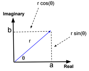
z = r (cos(θ) + i sin(θ))

Exponential form

z = r.exp(iθ)

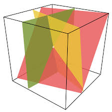
Multivariate equations

The solution set of a system of linear equations with 3 variables is the intersection of hyperplanes defined by each linear equation.

Derivatives

\(\frac{\partial f(x)}{\partial x} = \lim_{h \rightarrow 0} \frac{f(x+h) – f(x)}{h}\)

Function	Derivative
x^n	n * x^(n-1)
exp(x)	exp(x)
f o g (x)	g’(x) * f’ o g(x)
ln(x)	1/x
sin(x)	cos(x)
cos(x)	-sin(x)

Integration by parts

\(\int_{a}^{b} (f(x) g(x))’ dx = \int_{a}^{b} f'(x) g(x) dx+ \int_{a}^{b} f(x) g'(x) dx\)

Binomial theorem

\((x + y)^n = \sum_{k=0}^{n} C_n^k x^k y^{n-k}\)

Chain rule

Z = f(x(u,v), y(u,v))

\(\frac{\partial Z}{\partial u} = \frac{\partial Z}{\partial x} * \frac{\partial x}{\partial u} + \frac{\partial Z}{\partial y} * \frac{\partial y}{\partial u}\)

Entropy

Entropy measures the uncertainty associated with a random variable.

\(H(X) = -\sum_{i=1}^n p(x^{(i)}) log(p(x^{(i)}))\)

Example:

Entropy({1,1,1,1}) = 0

Entropy({0,1,0,1}) = -½ (4*log(½))

Hessian

\(H = \begin{bmatrix}\frac{\partial^2 f(θ)}{\partial θ_1\partial θ_1} & \frac{\partial^2 f(θ)}{\partial θ_1 \partial θ_2} \\ \frac{\partial^2 f(θ)}{\partial θ_2\partial θ_1} & \frac{\partial^2 f(θ)}{\partial θ_2\partial θ_2} \end{bmatrix}\)

Example:

\(f(θ) = θ_1^2 + θ_2^2 \\ H(f) = \begin{bmatrix} 2 & 0 \\ 0 & 2 \end{bmatrix}\)

A function f(θ) is convex if its Hessian matrix is positive semidefinite (\(x^T.H(θ).x >= 0\), for every \(x∈R^2\)).

\(x^T.H(θ).x = \begin{bmatrix} x_1 & x_2 \end{bmatrix} . \begin{bmatrix} 2 & 0 \\ 0 & 2 \end{bmatrix} . \begin{bmatrix} x_1\\ x_2 \end{bmatrix} = 2 x_1^2 + 2 x_2^2 >= 0\)

Method of Lagrange Multipliers

To maximize/minimize f(x) with the constraints \(h_r(x) = 0\) for r in {1,..,l},

We need to define the Lagrangian: \(L(x, α) = f(x) – \sum_{r=1}^l α_r h_r(x)\) and find x, α by solving the following equations:

\(\frac{\partial L}{\partial x} = 0\)

\(\frac{\partial L}{\partial α_r} = 0\) for all r

\(h_r(x) = 0\) for all r

Calculate the Hessian matrix (f”(x)) to know if the solution is a minimum or maximum.

Method of Lagrange Multipliers with inequality constraints

To minimize f(x) with the constraints \(g_i(x) \geq 0\) for i in {1,..,k} and \(h_r(x) = 0\) for r in {1,..,l},

We need to define the Lagrangian: \(L(x, α, β) = f(w) – \sum_{i=1}^k α_i g_i(x) – \sum_{r=1}^l β_r h_r(x)\) and find x, α, β by solving the following equations:

\(\frac{\partial L}{\partial x} = 0\)

\(\frac{\partial L}{\partial α_i} = 0\) for all i

\(\frac{\partial L}{\partial β_r} = 0\) for all r

\(h_r(x) = 0\) for all r

\(g_i(x) \geq 0\) for all i

\(α_i * g_i(x) = 0\) for all i (Karush–Kuhn–Tucker conditions)

\(α_i >= 0\) for all i (KTT conditions)

Lagrange strong duality – hard to understand 🙁

Lagrange dual function \(d(α, β) = \underset{x}{min} L(x, α, β)\), and x satisfies equality and inequality constraints.

We define \(d^* = \underset{α \geq 0, β}{max}\ d(α, β)\)

We define \(p^* = \underset{w}{min}\ f(x) \) (x satisfies equality and inequality constraints)

Under certain conditions (Slater conditions: f convex,…), \(p^* = d^*\)

Jensen’s inequality

If f a convex function, and X a random variable, then f(E[X]) <= E[f(X)].

If f a concave function, and X a random variable, then f(E[X]) >= E[f(X)].

If f is strictly convex (f”(x) > 0), then f(E[X]) = E[f(X)] holds true only if X = E[X] (X is a constant).

Probability

Below the main probability theorems.

Law of total probability

If A is an arbitrary event, and B are mutually exclusive events such as \(\sum_{i=1}^{n} P(B_{i}) = 1\), then:

\(P(A) = \sum_{i=1}^{n} P(A|B_{i}) P(B_{i}) = \sum_{i=1}^{n} P(A,B_{i})\)

Example:

Suppose that 15% of the population of your country was exposed to a dangerous chemical Z. If exposure to Z quadruples the risk of lung cancer from .0001 to .0004. What’s the probability that you will get lung cancer.

P(cancer) = .15 * .0004 + .85 * .0001 = .000145

Bayes’ rule

P(A|B) = P(B|A) * P(A) / P(B)

Where A and B are events.

Example:

Suppose that 15% of the population of your country was exposed to a dangerous chemical Z. If exposure to Z quadruples the risk of lung cancer from .0001 to .0004. If you have lung cancer, what’s the probability that you were exposed to Z?

P(Z|Cancer) = P(Cancer|Z) * P(Z) / P(Cancer)

We can calculate the P(Cancer) using the law of total probability: P(Cancer) = P(Cancer|Z) * P(Z) + P(Cancer|~Z) * P(~Z)

P(Z|Cancer) = .0004 * 0.15 / (.0004 * 0.15 + .0001 * .85) = 0.41

Chain rule

\(P(A_1,A_2,…,A_n) = P(A_1) P(A_2|A_1) ….P(A_n|A_{n-1},…,A_1)\)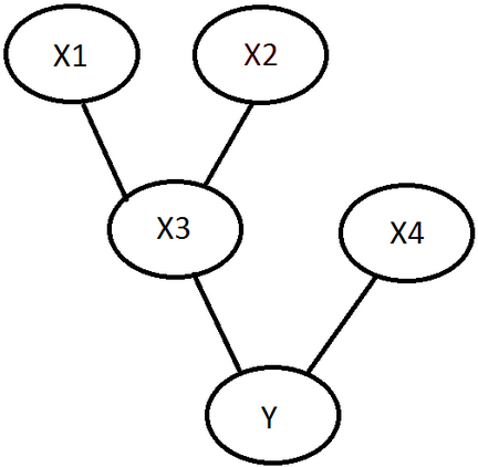

P(Y,X1,X2,X3,X4) = P(Y,X4,X3,X2,X1)

= P(Y|X4,X3,X2,X1) * P(X4|X3,X2,X1) * P(X3|X2,X1) * P(X2|X1) * P(X1)

= P(Y|X4,X3) * P(X4) * P(X3|X2,X1) * P(X2) * P(X1)

The Union Bound

\(P(A_1 \cup A_2 … \cup A_n) \leq P(A_1) + P(A_2) + … + P(A_n) \)

Nb of permutations with replacement

Nb of permutations with replacement = \({n^r}\), r the number of events, n the number of elements.

Probability = \(\frac{1}{n^r}\)

Example:

Probability of getting 3 six when rolling a dice = 1/6 * 1/6 * 1/6

Probability of getting 3 heads when flipping a coin = 1/2 * 1/2 * 1/2

Nb of permutations without replacement and with ordering

Nb of permutations without replacement = \(\frac{n!}{(n-r)!}\), r the number of events, n the number of elements.

Probability = \(\frac{(n-r)!}{n!}\)

Example:

Probability of getting 1 red ball and then 1 green ball from an urn that contains 4 balls (1 red, 1 green, 1 black and 1 blue) = 1/4 * 1/3

Nb of combinations without replacement and without ordering

Nb of combinations \(\frac{n!}{(n-r)! \, r!}\), r the number of events, n the number of elements.

Probability = \(\frac{(n-r)! \, r!}{n!}\)

Example:

Probability of getting 1 red ball and 1 green ball from an urn that contains 4 balls (1 red, 1 green, 1 black and 1 blue) = 1/4 * 1/3 + 1/4 * ⅓